


[Administrative note: Office hours for paid Bamboo Weekly subscribers will take place on Sunday. Come with any and all questions about Pandas! I’ll send a note with the Zoom link tomorrow.]
This week, we looked at data provided by the US government regarding “border encounters,” when officers from the Department of Homeland Security’s Customs and Border Protection (CBP) met people who hadn’t legally entered the United States.
The CBP classifies each of these encounters in one of three ways: Expulsion (i.e., the person is removed from the US without a hearing), apprehension (i.e., the person was found having entered the US illegally), or inadmissible (i.e., the person tried to enter at an established port of entry, but didn’t have the appropriate documentation).
My impression, based on reading the news, was that there was a recent, massive surge in people entering the US outside of standard ports of entry. Southern states have complained bitterly about the large number of people entering illegally — although according to US and international law, many people who are classified as “apprehension” or “inadmissible” are able to claim asylum or refugee status. In such cases, they then stay in the US until their case is heard before a judge.
Data and nine questions
This week’s data came from the CBP. The main source of data that they offer is a CSV file describing all border encounters since fiscal year 2021. (We’ll discuss fiscal years in detail, below.) There are also data files for pre-2021 border encounters, but my impression is that they were reported in a different way, and this was enough data for us to get a sense of the current trends.
The CSV file can be downloaded from the main CBP data page, at:
https://www.cbp.gov/document/stats/nationwide-encounters
The specific file that I asked you to download was for information from fiscal year 2021 through fiscal year 2024, ending in December of FY 2024:
A data dictionary, describing the different fields and values contained in the CSV file, was here:
Here are the nine questions and tasks that I gave you, with my detailed solutions and explanations. A link to the Jupyter notebook I used to perform the calculations follows my solutions:
Read the data from the CSV file into a data frame. Convert "2024 FYTD" into just "2024".
Before doing anything else, I loaded Pandas into Python:
import pandas as pdNext, I used “read_csv” to load the CSV file into a data frame:
df = (pd
      .read_csv(filename)
     )
However, I wanted to change values in the “Fiscal Year” column to “2024” from “2024 (FYTD)”, meaning “fiscal year to date.” I can understand why, before FY 2024 is complete, the data would indicate that it was incomplete. However, this would cause a lot of trouble in working with dates, and I decided to standardize it.
I decided to use the “replace” method on the data frame. There are several ways to invoke this method; one is to simply pass it a dictionary, in which case the dict’s key-value pairs tell Pandas what values should be replaced with other values. We could, in theory, have done just that — but I decided to use a more advanced feature of replace, focusing our search-and-replace operation to a particular column. Here, the dict’s key is “Fiscal Year,” and the value is a dict whose key-value pairs indicate the values to be found and replaced:
df = (pd
      .read_csv(filename)
      .replace({'Fiscal Year':{'2024 (FYTD)':'2024'}})
     )
Create a "date" new column, based on the "Fiscal Year" and "Month (abbv)" columns, containing a datetime value for that year and month based on the fiscal year. Make that the index.
It’s always nice when we get a pre-packaged date/time field in a CSV file. We can then pass the “parse_dates” keyword argument to read_csv, and get a datetime field.
In this case, though, we weren’t so lucky: We got separate columns for the year (well, the fiscal year) and for the month. How can we turn that into a datetime column?
One way is to use “pd.to_datetime”, a Pandas function that takes a series of strings and returns a series of datetime objects. If we can create a series of strings in a reasonable format, then we can call to_datetime on those values.
I decided to use “assign” to create the new column. I created the column by concatenating together (with “+”) the “Fiscal Year” and “Month (abbv)” columns, with a minus sign between them.
However, when I ran pd.to_datetime on the resulting string, I got some Pandas warnings that told me the format was ambiguous, and that I should specify it clearly by passing a format string.
Such format strings are commonly used with “strftime” and “strptime”, used for formatting and parsing date strings. You can read about the different format strings here:
https://docs.python.org/3/library/datetime.html#strftime-and-strptime-format-codes
The basic idea is that the string is taken literally except for % followed by particular letters. For example, %Y means a 4-digit year, and %b is the name of a month. By passing a format string of “%Y-%b”, we can tell Pandas to parse the dates we have created in our new column, resulting in a datetime dtype:
df = (
    df
    .assign(date = pd.to_datetime(df['Fiscal Year'] +
                                  '-' + df['Month (abbv)'],
                                  format='%Y-%b'))
)
Note that when you create a datetime object but only supply a year and month, the resulting datetime has the year and month you specified, with the day being the 1st of the month. The time component is similarly set to midnight.
With this date column in place, I then asked you to use it as the data frame’s index. We can use the “set_index” method to accomplish this:
df = (
    df
    .assign(date = pd.to_datetime(df['Fiscal Year'] +
                                  '-' + df['Month (abbv)'],
                                  format='%Y-%b'))
    .set_index('date')
)
We now have a data frame whose index contains datetime values. This is known as a “time series,” and it’s both common and very useful.
However, as we’ll soon see, there are some problems with using fiscal years as if they were calendar years.
Create a line plot showing, month by month, the total number of people caught by the US government. What's weird or wrong about this graph?
We have a column named “Encounter Count”, and we could get the total number of people by summing the column. However, we don’t want the total, per se. Rather, we want the total for each month. This means that we somehow need to break down our data set, calculating the sum for the rows in each month.
I can easily imagine using “groupby” for this, but when it comes to time series, I often prefer to use “resample”, which you can think of as a specialized version of groupby. We just need to tell resample the granularity that we want to use, namely per month. It used to be that we could indicate one-month granularity by stating “1M”, but in order to reduce ambiguity, we now say “1ME”, meaning “month end.” There is also a “MS” offset string, which indicates “month start.”
You can read about all of the resample offset strings here: https://pandas.pydata.org/pandas-docs/stable/user_guide/timeseries.html#dateoffset-objects
I can thus say:
(
    df
    .resample('1ME')['Encounter Count'].sum()
)
In other words: We want to take all of the rows in df, and sum up the values of “Encounter Count”, getting a result for each month in the system. The result is a series. I then asked you to plot this series, which we can do by applying “plot.line”:
(
    df
    .resample('1ME')['Encounter Count'].sum()
    .plot.line()
)
The result looks like this:
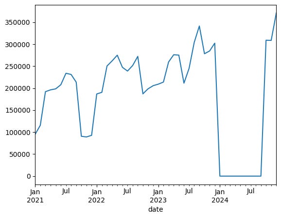
Could it possibly be that there were no border encounters at all from January 2024 until August 2024, when we suddenly see the numbers skyrocket? And wait… I’m writing this in February 2024, so doesn’t it seem a bit premature for us to be calculating the number of border encounters in October of this year?
We can explain this by taking into account the fact that this data uses fiscal years. I’ve never quite understood the need for fiscal years; in Israel, every company and the government goes from January 1st through December 31st. In the US, though, the government starts each fiscal year in October. That means FY October 2024 - FY December 2024 have already passed, because they were in October 2023 - December 2023. FY January 2024 also happened, but wasn’t included in our data set.
This is… annoying, to say the least. But that’s what happens when you treat fiscal years as calendar years.
Convert the index from using fiscal years to using calendar years. This means that any date in October, November, or December should have its year reduced by 1.
In order to better understand our data, I asked you to convert the dates from fiscal years to calendar years. This means that if the month is October, November, or December (i.e., months 10, 11, or 12), then we should subtract 1 from the year.
If we were simply interested in reducing the year by 1, we could just do so, probably using “datetime.replace”, a method in Python’s standard library that lets us perform this sort of calculation. But we don’t want to decrement all of the years in the index, just those for months 10, 11, and 12. We’ll thus need an “if” statement, which means a function of some sort.
Here’s a function that we could use, for example:
def fiscal_to_calendar(date):
    if date.month < 10:
        return date
    else:
        return date.replace(year=date.year - 1)
Notice how I used datetime.replace in the above code: I invoked “date.replace”, indicating that its year should be “date.year - 1”. In other words, I got a new date identical to the old one, except one calendar year earlier.
If this were a regular column or series, we could invoke this function with “apply”, running the function on each element of the series. But we have made our series into an index, which makes such things a bit trickier.
At first, I played with invoking “reset_index” on the data frame, applying a function to our “date” column, and then setting it to be the index again. But that seemed a bit much.
In the end, I realized that we can assign a list or other iterable to a data frame’s “index” attribute. Given that I wanted to iterate over the index, invoke a function on each element, and then get a new list — well, that sounded like a great use for list comprehensions. And indeed, this is what I came up with:
df.index = [fiscal_to_calendar(d)
            for d in df.index]
Sure enough, this performed the transformation that I wanted.
Rerun the plot from question 3. What sort of trend do you see?
Running the plot code again gave us a much more reasonable view of things:
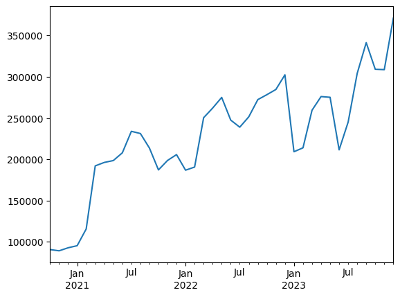
We can see that the number of border encounters has indeed been rising steadily. Yes, there was a major drop in January of 2023 (and to some degree in July 2022), but we see a larger and larger number of people being stopped and classified by CBP — such that the number now is more than 3x what it was in January 2021, about three years ago.
Now draw three lines on the same plot showing, over time, the total number of people caught by the US government in each of the three "Encounter Type" values.
If you invoke “plot.line” on a Pandas data frame, then you’ll get one line per column, with a shared x axis corresponding to the data frame’s index. How can we massage our data frame into that format?
Well, since we want to find out how many people were in each category, it makes sense that we’ll want to run “groupby” on “Encounter Type”:
(
    df
    .groupby('Encounter Type')
)
But…then what? How can we then sum them per month? Do we group by encounter type and month?
Here’s a neat trick: When we run “groupby”, we don’t get the results right away. Rather, we get a “groupby” object, on which we normally select one or more columns (with square brackets) and run an aggregation method.
But what if, instead of running an aggregation method right away, we were to run “resample”? We could resample by month, summing the values for “Encounter Count”:
(
    df
    .groupby('Encounter Type')
    .resample('1ME')['Encounter Count'].sum()
)
a
We get the following series back:
Encounter Type
Apprehensions   2020-10-31      6205
                2020-11-30      8042
                2020-12-31     10697
                2021-01-31     12983
                2021-02-28     25480
                               ...
Inadmissibles   2023-08-31    121696
                2023-09-30    121069
                2023-10-31    118631
                2023-11-30    116308
                2023-12-31    119814
Name: Encounter Count, Length: 110, dtype: int64
Notice that the series has a multi-index, with the outer part (level 0) being the encounter types, and the inner parts (level 1) being the dates. Since we’re grouping by month end, we’ll once again see the final day of each month as the inner index value.
But wait a second — this isn’t really what we wanted! We want to have a data frame with the dates as the index and the encounter types as the columns. Fortunately, we can use the “unstack” method, passing it the “level=0” keyword argument. That takes level 0 of our multi-index and turns it into columns:
(
    df
    .groupby('Encounter Type')
    .resample('1ME')['Encounter Count'].sum()
    .unstack(level=0)
)
Here’s (part of) what we see as a result:
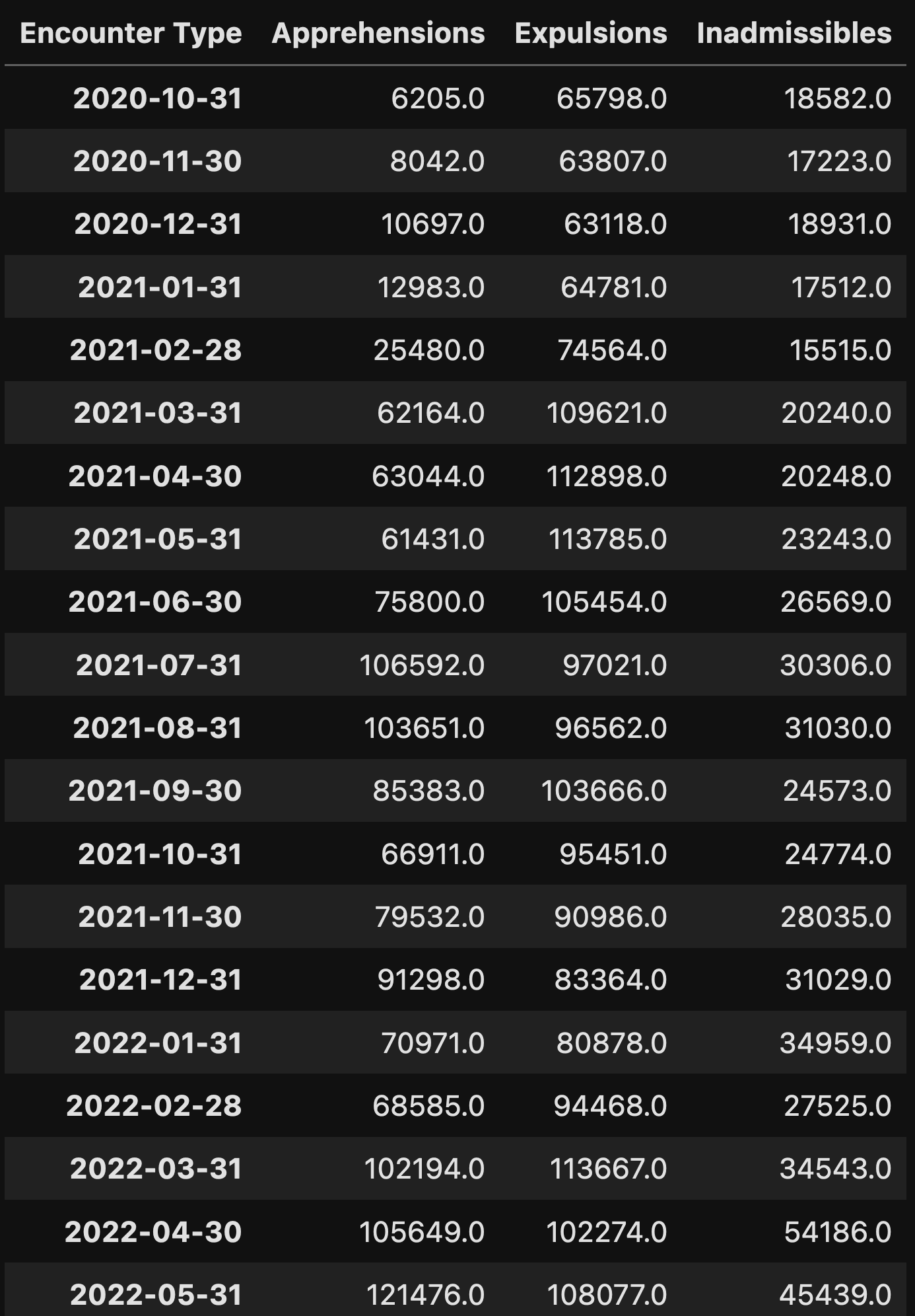
We have massaged our data into the format that we want to create our plot! Now all that’s left is to plot it:
(
    df
    .groupby('Encounter Type')
    .resample('1ME')['Encounter Count'].sum()
    .unstack(level=0)
    .plot.line()
)
The result:
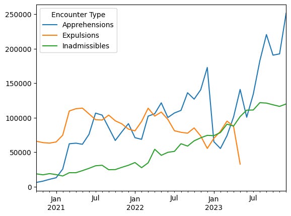
This plot makes it pretty clear that the number of apprehensions — that is, people who have encountered CBP entering the US outside of official locations and ports — has really skyrocketed in recent months, as southern governors have claimed. The number of expulsions has gone down quite a bit, as well.
You can see how this makes for a good political case against the Biden administration. Although you can also see how Biden and his team can use it against the Republicans, who just voted down their own proposals to fix some of these problems.
Create a data frame with one row for each country of citizenship reported by CBP, and one column for each year in the data set. The values should reflect the percentage of people from each country encountered in each year. (That is, each column should sum to 1.0.)
Now I want to find out what countries people are coming from, and I want to see that percentage per year. To get the information on an annual basis, I’ll once again use “resample”, this time using the “1YE” (end of one year) code. I’ll group on “Citizenship,” and will invoke “value_counts” as my aggregation method. This will have the effect of running value_counts on each distinct year in our data set.
However, value_counts normally gives us the raw numbers. We want to get percentages. Fortunately, we can pass “normalize=True” to value_counts, and thus get percentages:
(
    df
    .resample('1YE')['Citizenship'].value_counts(normalize=True)
)
However, we’ve once again gotten a series with a two-level multi-index:
            Citizenship
2020-12-31  MEXICO             0.127174
            OTHER              0.088768
            GUATEMALA          0.080072
            HONDURAS           0.073913
            EL SALVADOR        0.068116
                                 ...
2023-12-31  CANADA             0.031611
            ROMANIA            0.027598
            TURKEY             0.023832
            PHILIPPINES        0.023646
            MYANMAR (BURMA)    0.011113
Name: proportion, Length: 88, dtype: float64
To get this into a data frame, we’ll need to use “unstack” again:
(
    df
    .resample('1YE')['Citizenship'].value_counts(normalize=True)
    .unstack(level=0)
)
This is our result:
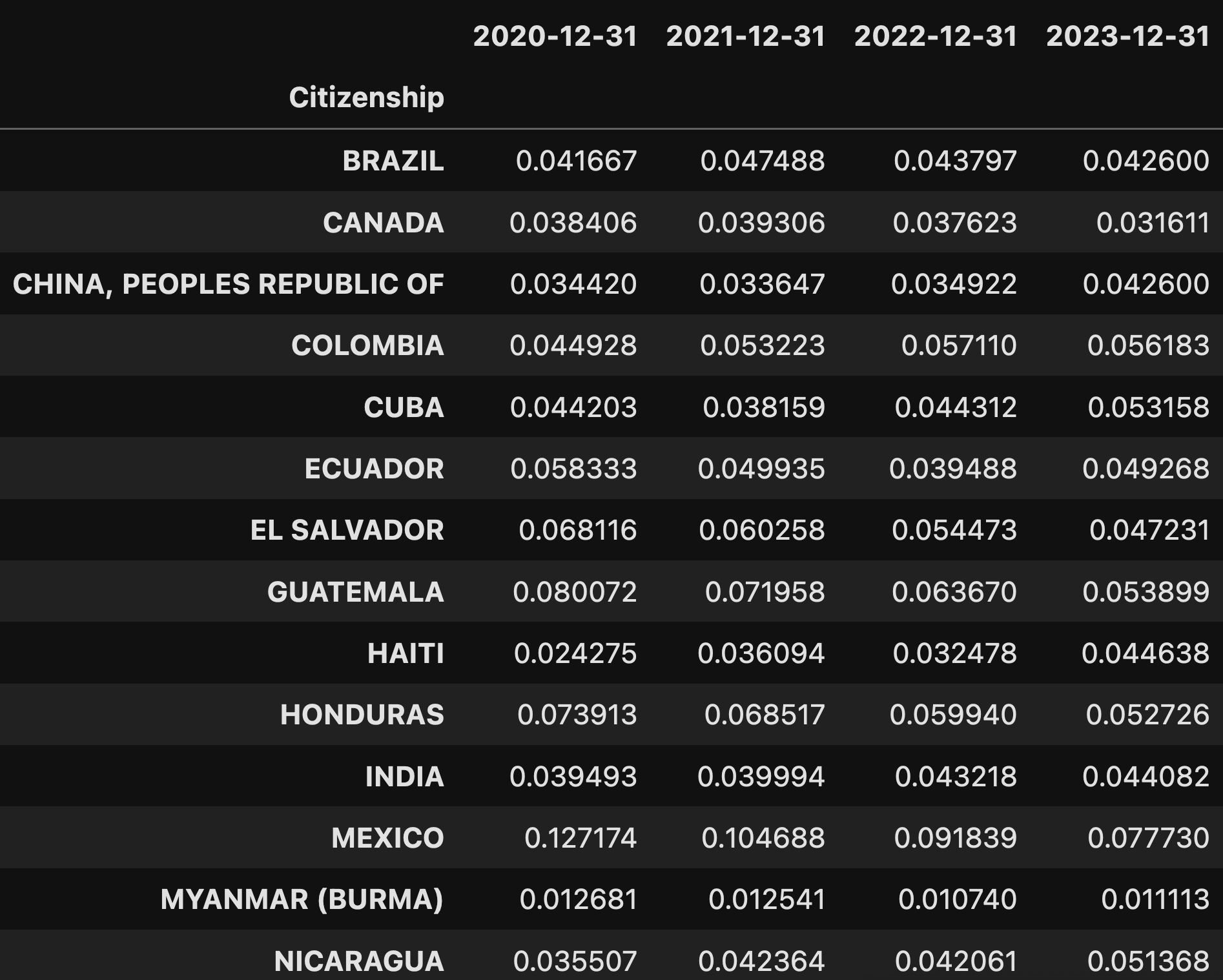
We now have the countries in our index, the years in our columns, and can see the percentage of people coming from each country in each year.
Calculate the degree by which these percentages have changed in the last year. Which countries have shown the greatest increase, as a percentage, in the number of people encountered by CBP? Which have shown the greatest decrease?
Now, instead of asking for annual percentages, I asked you to find the change in annual percentages, so that we can see if the mix of nationalities encountered by CBP is changing.
We can compare adjacent rows with a “window function.” The easiest window functions are “diff” and “pct_change”. In this case, we want to know the percentage change from year to year, so pct_change would seem to be the right thing to use.
The problem, though, is that pct_change works across rows. We want to calculate across columns. Fortunately, we can tell is to use “axis='columns'”, and the problem is solved:
(
    df
    .resample('1YE')['Citizenship'].value_counts(normalize=True)
    .unstack(level=0)
    .pct_change(axis='columns')
)
Now let’s look only at the most recent report. We can do that by selecting the column for “2023-12-31”:
(
    df
    .resample('1YE')['Citizenship'].value_counts(normalize=True)
    .unstack(level=0)
    .pct_change(axis='columns')
    ['2023-12-31']
)
Finally, we can sort the values from lowest to high:
(
    df
    .resample('1YE')['Citizenship'].value_counts(normalize=True)
    .unstack(level=0)
    .pct_change(axis='columns')
    ['2023-12-31']
    .sort_values()
)
Here’s what we get:
Citizenship
CANADA                       -0.159801
MEXICO                       -0.153620
GUATEMALA                    -0.153461
EL SALVADOR                  -0.132946
HONDURAS                     -0.120350
UKRAINE                      -0.108671
RUSSIA                       -0.100504
ROMANIA                      -0.094691
PHILIPPINES                  -0.062048
OTHER                        -0.052667
BRAZIL                       -0.027320
TURKEY                       -0.024850
COLOMBIA                     -0.016224
INDIA                         0.019992
MYANMAR (BURMA)               0.034723
PERU                          0.059513
CUBA                          0.199642
CHINA, PEOPLES REPUBLIC OF    0.219880
NICARAGUA                     0.221275
ECUADOR                       0.247678
VENEZUELA                     0.278332
HAITI                         0.374405
Name: 2023-12-31 00:00:00, dtype: float64
Note that we’re not saying that the number of Canadians encountered by CBP went down by 15.9 percent, or that the number of Haitians went up by 37.4 percent. Rather, we’re saying that their share of the total went up and down by that much. In other words, CBP officers are seeing proportionally more Haitians, Venezuelas, Ecuadorians, and Nicaraguans than they did last year.
We hear about unaccompanied minors coming from other countries into the United States. In 2023, from what 10 countries did the greatest number of unaccompanied minors enter the US?
Finally, the political discussion often mentions unaccompanied minors entering the US from other countries. I asked you to find out which 10 countries were the source of most unaccompanied minors entering the US.
First, I wanted to select only those rows from 2023. I used “loc”, and since the index contains datetime values, I could indicate “2023” and it returned only those rows from that year:
(
    df
    .loc['2023']
)
Next, I used another loc, this time with “lambda”, to retrieve only those rows in which the demographic was single minors. Notice that I used df_, a parameter, to perform my comparison on the result of the previous filter; if I had used “df”, then it would have included rows from outside of the year 2023:
(
    df
    .loc['2023']
    .loc[lambda df_: df_['Demographic'] == 'UC / Single Minors']
)
Next, I selected only the “Citizenship” column:
(
    df
    .loc['2023']
    .loc[lambda df_: df_['Demographic'] == 'UC / Single Minors']
    ['Citizenship']
)
I now had the “Citizenship” column for 2023, and only for unaccompanied and single minors. I counted them with value_counts, and then sorted them with sort_values:
(
    df
    .loc['2023']
    .loc[lambda df_: df_['Demographic'] == 'UC / Single Minors']
    ['Citizenship']
    .value_counts()
    .sort_values(ascending=False)
)
Here’s the result I got:
Citizenship
OTHER                         208
MEXICO                        193
GUATEMALA                     166
HONDURAS                      157
EL SALVADOR                   134
ECUADOR                       132
COLOMBIA                      119
VENEZUELA                     117
CUBA                          109
PERU                           92
NICARAGUA                      88
HAITI                          77
INDIA                          71
BRAZIL                         56
CANADA                         40
CHINA, PEOPLES REPUBLIC OF     39
RUSSIA                         30
ROMANIA                        21
TURKEY                         19
UKRAINE                        17
PHILIPPINES                     4
MYANMAR (BURMA)                 1
Name: count, dtype: int64
I have to assume that “other” doesn’t really mean other countries, but rather means that we don’t know, or didn’t have documentation. But many others came from Mexico, Guatemala, Honduras, El Salvador, and other countries in Latin America.
And that’s it for this week’s comparison!
My Jupyter notebook is here: https://drive.google.com/file/d/1MWr44CLyjoTAh4AX99oSs7NOKTw0FSba/view?usp=sharing
I’ll be back next week with more Pandas problems based on current events.
Until then,
Reuven