Bamboo Weekly #80: Inflation (solutions)

[Want to learn about Polars? On Sunday, I'll be teaching my first-ever course on Polars. You can buy the course on its own at https://store.lerner.co.il/polars, or get it as part of my Python+data membership at https://LernerPython.com. The membership includes my entire catalog of courses, as well as twice-monthly office hours, frequent members-only lectures, a private forum where you can ask Python+Pandas questions, and a paid membership to Bamboo Weekly. Any questions? Just e-mail me at reuven@lerner.co.il.]

This week, we looked at inflation. Specifically, we wanted to know whether it's still bad, and whether it's equally bad in all countries. There's all sorts of talk about the Federal Reserve reducing interest rates when it next meets, and there is talk about the European Central Bank taking a similar step next month. If true, that would mean inflation has subsided somewhat, and that central banks can try to (gently) push the economy toward greater expansion.

Normally, I ask you to use Pandas to analyze our data. But the Polars library (https://pola.rs/) continues to draw interest and mindshare from Pandas users. That's partly because of its speed, partly because of its very clean API, and partly because it can handle larger data sets via lazy execution. Even if you won't use Polars, it's important to know how it works and how to use it, because its design will certainly come back to influence Pandas and other data-analysis libraries.

Data and six questions

This week's data come from the OECD (Organisation for Economic Co-operation and Development, https://www.oecd.org/), which the Economist calls a "club of mostly-rich countries."

I downloaded the inflation data from the OECD's data explorer:

https://data-explorer.oecd.org/vis?tm=inflation&pg=0&snb=50&df[ds]=dsDisseminateFinalDMZ&df[id]=DSD_G20_PRICES%40DF_G20_PRICES&df[ag]=OECD.SDD.TPS&df[vs]=1.0&dq=.M...PA...&lom=LASTNPERIODS&lo=13&to[TIME_PERIOD]=false

You can view and play with the data there, in your browser. But you can also download the data in CSV format, either by clicking on the "download" button, or by using this URL:

https://sdmx.oecd.org/public/rest/data/OECD.SDD.TPS,DSD_G20_PRICES@DF_G20_PRICES,1.0/all?dimensionAtObservation=AllDimensions&format=csvfilewithlabels

This week, I gave you six questions and tasks to answer with Polars. Here are my detailed solutions; as usual, a link to my downloadable Jupyter notebook is at the end of this post.

Create a data frame from the CSV file. Keep only those columns containing ALL CAPS.

Before we can do anything else, we'll need to load up Polars. You can install it via pip:

pip install polars

Two quick caveats, though:

1. I use a Mac, and installed Python using pyenv. The version that I installed apparently runs in Intel compatibility mode, which resulted in errors when I tried to import polars. I installed a variant of Polars, polars-lts-cpu, and the errors went away.
2. Because I'm constantly experimenting with packages, I installed all of the dependencies along with Polars. To do that, I used pip install 'polars-lts-cpu[all]', combining the fixes that I needed with a bunch of other packages.

Once you have Polars installed, you can import it. Just as Pandas as a standard alias of "pd", Polars has a standard alias of "pl":

import polars as pl

With that in place, we can then work with the CSV file that I downloaded from the OECD.

filename = 'OECD.SDD.TPS,DSD_G20_PRICES@DF_G20_PRICES,1.0+all.csv'

df = pl.read_csv(filename)

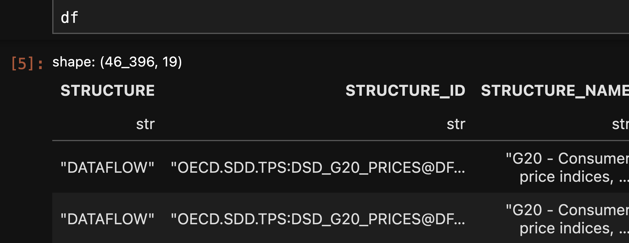
At this point, we now have a data frame, one which looks and feels much like a Pandas data frame. But there are differences, the biggest one being the lack of an index. Polars data frames have no index; instead, you use any column, along with an expression, to select rows.

However, the data frame does have columns, and each column has a unique name. Looking at our Polars data frame, we also see the dtype for each column at the top. (You can also run df.dtypes to get the full list of dtypes.) In this data frame, much of the data is repeated, with ALL_CAPS columns containing shorter forms, and Long_names containing longer forms.

I asked you to keep only those columns with ALL_CAPS names. As in Pandas, we can pass a data frame a list of column names inside of [] to get back a new data frame with a subset of the original columns. So in theory, I could run df.columns, getting the column names, edit that list by hand to remove mixed-case names, and then pass the resulting list to df.

But there's an easier way, namely a list comprehension: I can pass it df.columns, and then only get back values where the column name is the same as the name after running via str.upper. I can then pass the resulting list to df, and assign it back to df:

df = df[[one_column_name
 for one_column_name in df.columns
 if one_column_name == one_column_name.upper()]]

The result is a data frame with 46,396 rows and 19 columns. You can actually see a data frame's shape whenever it's displayed on the screen:

Remove rows in which the location is EA20, EU27_2020, or G20.

We're interested in per-country inflation, but the OECD data includes statistics about a number of country groupings – the EA20 (the 20 "Eurozone" countries that use the euro as their currency), EU27_2020 (the 27 members of the European Union, following the United Kingdom's exit in 2020), and the G20 (19 countries, the European Union, and the African Union). Those are certainly interesting and important, but I asked you to remove them from the data frame.

To select rows in Polars, we create an expression describing what we want to see, and then hand it to the filter method. But how do we create such an expression?

Assuming that it'll have to do with a column – and that's often going to be the case – we can select it by running the pl.col function. (This is technically a class, and every time we invoke pl.col, we're getting an instance of the Col class. But if they call it a function, then I feel OK doing so, too.) We pass pl.col the name of the column we want to use as a string; in this case, that'll be REF_AREA.

But then what? How can we indicate that we want rows that aren't equal to any of these three values?

One way would be to create three pl.col expressions, and & them together inside our call to pl.filter:

(
    df
    .filter(
        (pl.col('REF_AREA') != 'EA20') &
        (pl.col('REF_AREA') != 'EU27_2020') &
        (pl.col('REF_AREA') != 'G20')
    )
)

Here, we use Python's inequality operator != three times, once for each of the string. These three expressions are combined and handed to pl.filter, and the result is a data frame in which all of the REF_AREA values represent countries, rather than groups of countries.

There's nothing wrong, per se, with filtering like this. But perhaps there's a way to tell Polars that we don't want rows with any of these three strings in REF_AREA?

Indeed there is, the is_in method. We can pass is_in a list of values, and the expression will return True if the column contains one of these values:

df = (
    df
    .filter(
    (pl.col("REF_AREA").is_in(['EA20', 'EU27_2020', 'G20']))
    )
)

This is great, except that it's the opposite of what we want: We actually want to remove such rows, not keep them.

To flip the logic of our expression, we use the ~ operator. NumPy and Pandas both use this operator in the same way, turning True into False and vice versa. We can thus say:

df = (
    df
    .filter(
    (~pl.col("REF_AREA").is_in(['EA20', 'EU27_2020', 'G20']))
    )
)

The result is a data frame in which REF_AREA doesn't have these three groupings, but does have all of the country information.

Find the percentage change in monthly inflation rate for the US in months starting in 2020. Sort by year and month.

To do this, we'll first need to find the rows that match these criteria. This will mean calling pl.col four times:

• Once for the US
• Once for monthly
• Once for the percentage change
• Once for dates in 2020 and beyond

Once again, we'll invoke pl.filter. The first three criteria, strung together with &, are similar to what we did before:

(
    df
    .filter(
        (pl.col('FREQ') == 'M') &
        (pl.col('REF_AREA') == 'USA') &
        (pl.col('UNIT_MEASURE') == 'PC') 
    )
)

But how can we keep only those dates in 2020 and beyond? The TIME_PERIOD column doesn't even have a datetime (or similar) dtype, so it seems particularly tricky.

Because the TIME_PERIOD column has a string dtype, we can access and run a number of string methods on it via the str accessor, similar to how we do it in Pandas. In this case, the accessor is even identical to what we would do in Pandas; we invoke str.contains, and then pass a regular expression describing what we want.

Since TIME_PERIOD is in the form YYYY-MM, we can just look for any string that starts with 202, and we'll be fine. We can indicate that the pattern needs to be anchored to the front of the string with ^, and then add this filtering statement:

(
    df
    .filter(
        (pl.col('FREQ') == 'M') &
        (pl.col('REF_AREA') == 'USA') &
        (pl.col('UNIT_MEASURE') == 'PC') &
        (pl.col('TIME_PERIOD').str.contains('^202'))
    )
)

Next, I decided to pare down the data frame, passing a list of column names (TIME_PERIOD and OBS_VALUE) inside of []. With only two columns left, I then sorted the data frame, using the sort method, by the TIME_PERIOD column:

(
    df
    .filter(
        (pl.col('FREQ') == 'M') &
        (pl.col('REF_AREA') == 'USA') &
        (pl.col('UNIT_MEASURE') == 'PC') &
        (pl.col('TIME_PERIOD').str.contains('^202'))
    )
    [['TIME_PERIOD', 'OBS_VALUE']]
    .sort('TIME_PERIOD')
)

The result:

shape: (55, 2)
┌────────────┬──────────┐
│ TIME_PERIOD ┆ OBS_VALUE │
│ ---         ┆ ---       │
│ str         ┆ f64       │
╞════════════╪══════════╡
│ 2020-01     ┆ 0.387977  │
│ 2020-02     ┆ 0.2740618 │
│ 2020-03     ┆ -0.217645 │
│ 2020-04     ┆ -0.668694 │
│ 2020-05     ┆ 0.00195   │
│ …           ┆ …         │
│ 2024-03     ┆ 0.646417  │
│ 2024-04     ┆ 0.3893293 │
│ 2024-05     ┆ 0.1661628 │
│ 2024-06     ┆ 0.033751  │
│ 2024-07     ┆ 0.1161773 │
└────────────┴──────────┘

Similar to Pandas, Polars will only show us the first few and last few rows of a data frame if it's larger than a handful of rows. If we're interested in seeing just the 10 most recent readings, we can add a call to tail(20) to our query:

(
    df
    .filter(
        (pl.col('FREQ') == 'M') &
        (pl.col('REF_AREA') == 'USA') &
        (pl.col('UNIT_MEASURE') == 'PC') &
        (pl.col('TIME_PERIOD').str.contains('^202'))
    )
    [['TIME_PERIOD', 'OBS_VALUE']]
    .sort('TIME_PERIOD')
    .tail(10)
)

The result:

shape: (10, 2)
┌────────────┬──────────┐
│ TIME_PERIOD ┆ OBS_VALUE │
│ ---         ┆ ---       │
│ str         ┆ f64       │
╞════════════╪══════════╡
│ 2023-10     ┆ -0.038338 │
│ 2023-11     ┆ -0.201514 │
│ 2023-12     ┆ -0.099332 │
│ 2024-01     ┆ 0.5447504 │
│ 2024-02     ┆ 0.6189672 │
│ 2024-03     ┆ 0.646417  │
│ 2024-04     ┆ 0.3893293 │
│ 2024-05     ┆ 0.1661628 │
│ 2024-06     ┆ 0.033751  │
│ 2024-07     ┆ 0.1161773 │
└────────────┴──────────┘

We can see that monthly inflation rates have indeed dropped quite a bit in the last year alone, precisely the effect that the Fed has aimed to produce. The danger was that raising interest rates too high would raise unemployment, but it remains extremely low, making the chances of an interest-rate cut in September that much higher.

By the way, we could also have used the top_k method, which would have given us the same results, albeit in reverse order:

(
    df
    .filter(
        (pl.col('FREQ') == 'M') &
        (pl.col('REF_AREA') == 'USA') &
        (pl.col('UNIT_MEASURE') == 'PC') &
        (pl.col('TIME_PERIOD').str.contains('^202'))
    )
    [['TIME_PERIOD', 'OBS_VALUE']]
    .top_k(10, by='TIME_PERIOD')
  )

Which five countries had the lowest percentage annual inflation in 2023? Which five had the highest?

Next, I asked you to find which countries had the lowest annual percentage inflation in 2023. (Data for 2024 is still coming in, month by month.)

This query is quite similar to the one we just did. The big difference is that we'll be looking at an annual frequency (A), the annual percentage (PA), and that the string contains (or starts with, if you prefer) 2023.

After filtering those rows, we can then pare down the data frame to the REF_AREA and OBS_VALUE columns, sort by OBS_VALUE , and invoke head to get the countries with the lowest inflation in 2023:

(
    df
     .filter(
        (pl.col('FREQ') == 'A') &
        (pl.col('UNIT_MEASURE') == 'PA') &
        (pl.col('TIME_PERIOD').str.contains('2023') )
     )   
    [['REF_AREA', 'OBS_VALUE']]
    .sort('OBS_VALUE')
    .head(5)
)

The result:

shape: (5, 2)
┌─────────┬──────────┐
│ REF_AREA ┆ OBS_VALUE │
│ ---      ┆ ---       │
│ str      ┆ f64       │
╞═════════╪══════════╡
│ CHN      ┆ 0.2       │
│ SAU      ┆ 2.327085  │
│ KOR      ┆ 3.597456  │
│ IDN      ┆ 3.669401  │
│ CAN      ┆ 3.879002  │
└─────────┴──────────┘

We see that China had low inflation (but they have other big problems), followed by Saudi Arabia, South Korea, Indonesia, and Canada. What about countries with high inflation? How can we get that? One option would be to run the same query, and then run tail instead of head. But we can also call sort with descending=True, flipping the default:

(
    df
     .filter(
        (pl.col('FREQ') == 'A') &
        (pl.col('UNIT_MEASURE') == 'PA') &
        (pl.col('TIME_PERIOD').str.contains('2023') )
     )   
    [['REF_AREA', 'OBS_VALUE']]
    .sort('OBS_VALUE', descending=True)
    .head(5)
)

By the way, notice two things about sort in Polars:

• First, Pandas has both sort_index and sort_values, because we might want to sort by the index, and we might want to sort by the values. Polars data frames have no index, so there's only one sort method.
• Second, sort methods in Pandas default to sorting in ascending order. If you want to make them sort in descending order. you pass ascending=False. Polars has the same default, namely ascending order, but you reverse it by saying descending=True, for the same effect, but precisely the opposite semantics.

As for the countries with the highest inflation? Argentina, Turkey, the UK, South Africa, and Germany. It's no surprise that in all of these countries, the ruling party either lost their most recent election, came close to doing so, or is just generally unpopular.

Create a pivot table in which the years (2010 and onward) are the columns, the country names are the rows, and the values contain the percentage annual inflation.

To create such a table, we'll first need to (again) filter the rows, keeping only those that we want:

(
    df
     .filter(
        (pl.col('FREQ') == 'A') &
        (pl.col('UNIT_MEASURE') == 'PA') &
        (pl.col('TIME_PERIOD').str.contains('^20[12]') )
     )       
)

In the above query, we keep the annual frequency, annual-percentage measure, and years that start with 201 or 202. The [12] in our string is a "character class" in a regular expression, meaning that we want one (but not both) of the characters to match.

But now that we've kept only the rows we want, how can we turn this into a pivot table? The pivot method, which requires that we pass the name of one categorical column for the columns, another for the rows, and a third (numeric) column for the values. By default, the mean method will be run on these values, but we can (if we want) specify something else. Here's what I ran:

(
    df
     .filter(
        (pl.col('FREQ') == 'A') &
        (pl.col('UNIT_MEASURE') == 'PA') &
        (pl.col('TIME_PERIOD').str.contains('^20[12]') )
     )       
    .pivot(on='TIME_PERIOD',
           index='REF_AREA',
           values='OBS_VALUE')
)

Here's a screenshot of what I got:

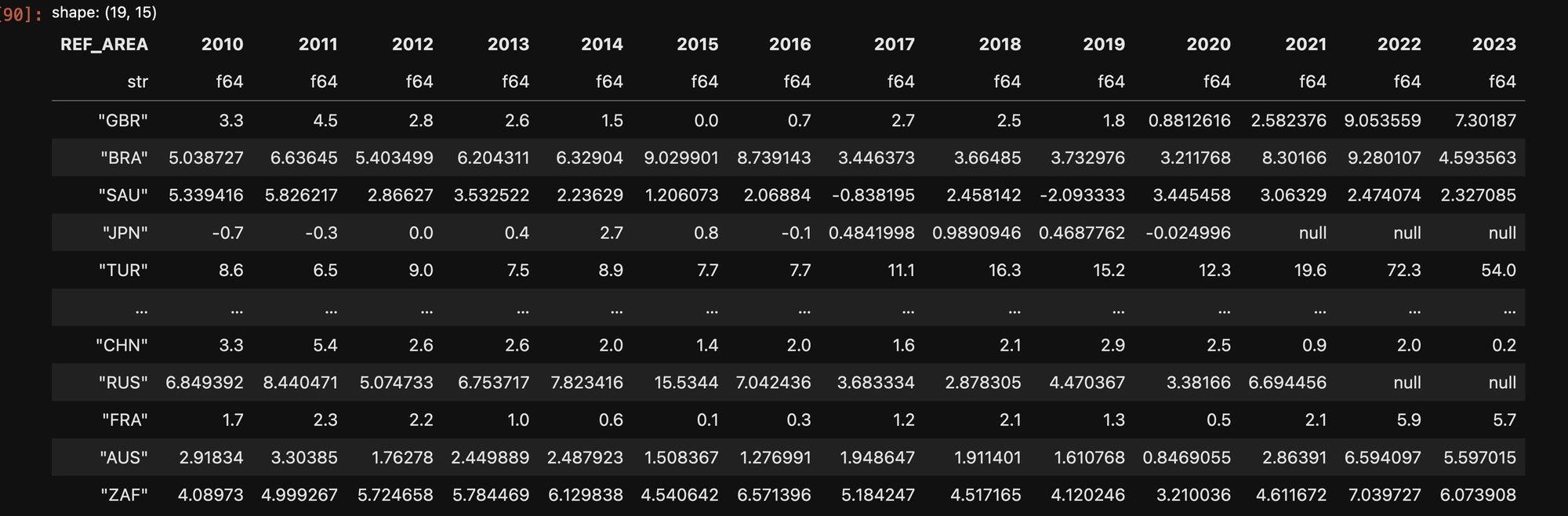
Notice that our data frame still doesn't have an index, per se. But the first column serves as one. Also notice that the data frame isn't sorted; I decided to add a sort('REF_AREA) to my notebook, just to make it a bit more aesthetic.

We can see that inflation in the US, and many other countries, was pretty steady for years, then jumped up in 2021-2022, and is now on its way down. Which doesn't mean that prices are lower than they were in 2021. Rather, it means that the rate of price increases has slowed dramatically.

What is the average annual inflation percentage for each country in the years 2020 and onward?

Finally, I asked you to get the average inflation percentage per country over the last few years. Now, looking at average inflation numbers is almost always a bad idea, especially in the last few years, when it has gone up and then (mostly) gone down. So this isn't a serious economic analysis. It is, however, a good way to introduce you to grouping in Polars.

We'll start by filtering on the rows we want:

(
    df
     .filter(
        (pl.col('FREQ') == 'A') &
        (pl.col('UNIT_MEASURE') == 'PA') &
        (pl.col('TIME_PERIOD').str.contains('^202') )
     )       
)

Next, we'll run a group_by operation. In Pandas, we need to say what categorical column we're grouping by, as well as the column(s) on which we want to run an aggregation method and the method itself.

In Polars, we do it a bit differently: We first run group_by, specifying the categorical column. We then invoke agg, passing it the column on which we want to calculate. Finally, we pass the mean method to the result of that.

Following that, we can sort by OBS_VALUE, much as we've done before.

The final query looks like this:

(
    df
     .filter(
        (pl.col('FREQ') == 'A') &
        (pl.col('UNIT_MEASURE') == 'PA') &
        (pl.col('TIME_PERIOD').str.contains('^202') )
     )       
    .group_by('REF_AREA').agg(pl.col('OBS_VALUE').mean())
    .sort('OBS_VALUE')
)

That's it for this week's queries.

You can see the Jupyter notebook I used here: https://drive.google.com/file/d/1Hs1CLjVIQwxcV_IQ_IdHUP19XFIE17kd/view?usp=sharing

I'll be back next week with more exercises in data analysis using Pandas (and friends).

Reuven