This week, we looked at a recent report from the US Census Bureau about poverty in the United States. The Census Bureau has been reporting on poverty for decades, not only keeping track of how many people are below the poverty line but also details about their race/ethnicity, age, level of education, marital status, and location.

The study came to my attention in a New York Times article from several days ago, "Poverty Rate Soared in 2022 as Aid Ended and Prices Rose", which confirmed some of the predictions that poverty experts had made several years ago — namely, that laws passed in 2020 and 2021 had made a huge impact on child poverty, and that the fact they weren’t renewed led to an uptick in child poverty afterward. Here’s an article from last year indicating how these laws reduced child poverty: https://www.vox.com/2022/9/14/23352022/child-poverty-covid-tax-credit

When I read such an article, I immediately ask myself where and how I can find the underlying data. Fortunately, the Census Bureau and other US government organizations make their findings public, and that’s the data that I decided we would look at this week.

If you’re interested in learning more about these poverty statistics, you can check out the Census Bureau's page describing the study is at https://www.census.gov/library/publications/2023/demo/p60-280.html , and a full report at /content/files/content/dam/Census/library/publications/2023/demo/p60-280.pdf .

From Stable Diffusion: “money disappearing gradually over time”

Data and eight questions

This week, I asked you eight questions about poverty. The questions were based on a single Excel file:

/content/files/programs-surveys/demo/tables/p60/280/tablea3_hist_pov_by_all_and_age.xlsx

The Census Bureau split their data across a number of different Excel files, all of which can be found and downloaded from:

https://www.census.gov/library/publications/2023/demo/p60-280.html

Here are the questions and tasks for this week, followed by a link to the Jupyter notebook that I used to solve things. Comments, corrections, and questions are, as always, welcome:

Read the "History POV by all and age" file into a data frame. We're only interested (for now) in the "ALL RACES" section. Turn the years into an index, and remove the "percent" measures.

Let’s start off by loading Pandas:

import pandas as pd

In theory, you can just say “import pandas”, and I in fact did that for my first year or two using Pandas. However, the fact that everyone in the Pandas world uses the “pd” alias means that if you don’t do it, you’ll find it hard to copy from Stack Overflow, blogs, or elsewhere. So even if you type quickly, it’s worth using “from .. import” when loading Pandas.

It’s tempting to say that you can just load the entire Excel file into a Pandas data frame with the “read_excel” function. However, there are several problems with this, chief among them being that the spreadsheet isn’t really just a glorified CSV file:

Rows 1-2 are a headline
Row 3 is a description
Rows 4-6 are headers for the data
Rows 7-73 contain data for all races, with row 7 being a headline, “ALL RACES”
Rows 74-97 contain data for “WHITE ALONE” race, including row 74 itself, a headline
Column A sometimes contains a year, sometimes contains a year and a footnote number, and sometimes contains a description of the data that follows
This continues for several more races/ethnicities until we get to row 482, where we’re told that “N” represents unavailable data
Rows 483 and onward are the footnotes references in the data (particularly the years)

It isn’t too hard for a human to make sense of this Excel file. But if we want to read the data into Pandas and make some sense of it, we’ll need to carve up the document when we read it. Otherwise, our data frame won’t make any sense, and certainly won’t have clear or useful dtypes in each of the columns.

Where do we even start? For the first few questions, we’re only interested in the “ALL RACES” part of the spreadsheet. That means rows 8-73, since row 7 is just the subtitle for that section of the document. We also want rows 4-6 to be our headers.

Of course, while Excel starts to number rows with 1, Python and Pandas people start to number things with 0. This means that from a Pandas perspective, we’ll want the headers to be from rows 3, 4, and 5, and the data to be for 67 rows starting after them. We can take an initial stab with this code:

filename = 'tableA3_hist_pov_by_all_and_age.xlsx'

df = (
    pd.read_excel(filename,
                  header=[3,4,5],
                  nrows=67)
)

I could have just assigned the result of pd.read_excel to the “df” variable, I’m planning to chain a bunch of additional methods to that result. I’m thus using a style of Pandas coding that Matt Harrison has promoted, and which I’m slowly but surely warming up to. We can get away with this because when you open a set of parentheses in Python, suddenly individual lines are all handled together; no longer is the end of a line considered the end of your Python statement.

This works, but we still have the “ALL RACES” row in our first row. That’ll throw off any dtype we try to use for the first column. We’ll thus want to remove that first row. We can do that with the “drop” method:

df = (
    pd.read_excel(filename,
                  header=[3,4,5],
                  nrows=67)
    .drop(0)
)

This works, but if you examine the data closely, you’ll see that in the final rows, we have the single-character string “N” in a number of places. That “N” is supposed to represent missing values, what we in the Pandas world would call either “NaN” or “NA”. If we can get those “N” values to be either NaN or NA, then Pandas will know what to do. But keeping them as “N” will prevent us from doing any calculations with those numbers.

The solution is to tell “read_excel” that when it sees “N”, it should treat it as a NaN value. We can do that with the “na_values” keyword argument. That argument can get a single string (as we’ll do here), or a list of values that should all be interpreted as NaN:

df = (
    pd.read_excel(filename,
                  header=[3,4,5],
                  nrows=67,
                 na_values='N')
    .drop(0)
)

At this point, the index of our data frame is a simple integer range, starting with 0. Our columns, however, are a multi-index with three levels, corresponding to rows 4, 5, and 6 in Excel. I asked you to remove the “Percent” part of the third level. (We’ll calculate those percentages ourselves.)

How can you do this? Dropping part of a multi-index shouldn’t be that hard, but dropping a subset of a level of a multi-index seems rather difficult. And yet, thanks to the “drop” method allows us to specify that we want to drop anything called “Percent” on level 2 in the columns:

df = (
    pd.read_excel(filename,
                  header=[3,4,5],
                  nrows=67,
                 na_values='N')
    .drop(0)
    .drop('Percent', axis='columns', level=2)
)

Once we have done that, we still have a three-level multi-index on our columns. However, “Below poverty” no longer has two sub-indexes under it (“Number” and “Percent”); it only has one (“Number”).

This is a good place to remind you that “drop”, like many methods in Pandas, doesn’t modify the original data frame. Rather, it returns a new data frame with the changes we’ve asked for. We can assign the result of the method call to a variable, or we can call an additional method on it, as I’ve done here. You could, in theory, use the “inplace=True” keyword argument on drop to modify the existing data frame, but we’re strongly urged not to do that by the core Pandas developers.

Next, I want to make the year into the index. This turns out to be quite tricky, because so many of the years have footnotes attached. In Excel, those footnotes are available as superscript integers, and are clearly visible. But when read into Pandas, those footnotes become part of the integer! The first five years, as read into Pandas, will thus be 2022, 2021, 20201, 2019, and 2018. And no, that third number isn’t a typo; it’s the year 2020 with footnote number 1 mashed together. Yuck.

I figured that I might be able to use the “str” accessor in Pandas to invoke the “slice” method on each of these numbers, grabbing only the first four digits. But in order to do that, I need to turn the column into a bunch of strings. And in order to do that, I need to grab the column, which is a pain because of its long name and the fact that we have a multi-index.

I thus decided to use “assign” to create a new column, called “Year”. While you can pass a single scalar value to an assign keyword argument, or you can pass a list/series of values, here I decided to pass a function object via “lambda”. The lambda will:

Use “df_” as its parameter, since it’s a temporary data frame
Grab the column names from the data frame’s “columns” attribute
Use the 0-index column name to retrieve the hard-to-write column name
Use “astype” to get a new series based on that column, all strings
Invoke the “str.slice” method, getting only the first 4 characters
Again invoke “astype”, this time getting back an integer

Once I’ve got that new “Year” column, I can invoke “set_index” to turn it into our data frame’s index. And now my data frame has an index containing integers, the years (sans footnote numbers) from that first column:

filename = 'tableA3_hist_pov_by_all_and_age.xlsx'

df = (
    pd.read_excel(filename,
                  header=[3,4,5],
                  nrows=67,
                 na_values='N')
    .drop(0)
    .drop('Percent', axis='columns', level=2)
    .assign(Year=lambda df_: df_[df_.columns[0]].astype(str).str.slice(None, 4).astype(int))
    .set_index('Year')
)

This is great, but we aren’t quite done: There’s no more need for that second (bottom) row in our multi-index of columns, so we can drop that. Here, I’ll use the “droplevel” method to get rid of level 2 from our multi-index. That returns a new multi-index data structure, which I can then assign back to “df.columns”.

df.columns = df.columns.droplevel(2)

I then (finally) get rid of the annoyingly named first column, which I don’t need any more because I have the years in an index:

df = df.drop(df.columns[0], axis='columns')

Why did I use assignment for these final two actions, rather than keep chaining methods? I didn’t see an obvious way to use method chaining, and I searched — but if you have suggestions, please add them in comments. As I always say, Pandas is huge and complex, and I’m constantly discovering new functionality and techniques.

Once we’re done with all of this, we have a data frame with 66 rows and 8 columns.

By the way, if you’re wondering why I didn’t use the “skiprows” keyword argument to “read_excel”, that was my first instinct, to skip over a bunch of rows. But that didn’t play well with the multi-index for columns that we got from the spreadsheet. Another option would have been to

In 2022, what was the number of Americans living below the poverty line?

It’s easy, when looking at poverty data, to think in terms of percentages, and changes in those percentages over time. We can feel good when the number of poor people goes down, and bad when that number goes up.

But percentages can mask actual numbers. I thus asked myself, and you: How many people in the United States are currently living below the poverty line?

The most recent year in the survey is 2022. Since we have set our index to contain years, we can retrieve the row for 2022 with the “loc” accessor:

df.loc[2022]

This returns the entire row whose index is 2022 as a series. The index for the series will be taken from our columns, meaning that we end up with a multi-indexed series:

All people         Total            330100.0
                   Below poverty     37920.0
Under 18 years     Total             71950.0
                   Below poverty     10780.0
18 to 64 years     Total            200200.0
                   Below poverty     21240.0
65 years and over  Total             57880.0
                   Below poverty      5897.0
Name: 2022, dtype: float64

How can we get the data for all people? “loc” takes two arguments, the first of which is a row selector (which is covered with 2022). The second, optional argument is a column selector, which can specify the column(s) we want. I could just say “All people”:

df.loc[
    2022,
    'All people'
]

Notice, by the way, that I like to use “loc” in this expanded, two-line form, so that we can separate the row selector from the column selector.

But the result that I get is a series, reflecting the two elements of the multi-index below “All people”:

Total            330100.0
Below poverty     37920.0
Name: 2022, dtype: float64

How can I say that I just want “All people”, and then “Below poverty” under that? I have to use a tuple:

df.loc[
    2022,
    ('All people', 'Below poverty')
]

My row selector remains 2022, but my column selector is a tuple, indicating what values I want in the primary and secondary parts of the multi-index.

The number I get back is 37920.0. Which is fine, but … that seems a bit low, no? Right, because (as it says at the top of the spreadsheet) all of the numbers describe a population in thousands. In other words, to get the real number of poor Americans in 2022, we need to multiply the result by 1,000:

df.loc[
    2022,
    ('All people', 'Below poverty')
] * 1000

The result is thus not 37920, but rather 37,920,000.

In other words: In 2022, there were nearly 38 million Americans living under the poverty line. I don’t know about you, but to me that’s a shockingly high number of people, more than 3x the entire population of Israel, where I live.

I don’t have any brilliant suggestions or solutions to offer, but it shows just how vast the scope of this problem is, and how many people are affected by poverty on a day-to-day basis in one of the world’s wealthiest countries.

Now calculate the percentage of all people below the poverty line in each year. In what year(s) was it highest and lowest?

Earlier, we got rid of the “Percentage” columns. Now, I want us to calculate the percentage of people living below the poverty line. To do this, we’ll need to divide the number of people below the poverty line by the total number of people.

Fortunately, this kind of calculation is pretty easy to do with Pandas:

df[('All people', 'Below poverty')] / df[('All people', 'Total')]

Once again, we need to use a tuple in order to specify which values we want from a multi-indexed column. Both of these values are under “All people,” but the first column is then “Below poverty,” and the second is “All people.” Notice that I’m using /, the “truediv” operator, which returns a float; if you want to get integer values back, you can use “//”, also known as “floordiv,” which removes any decimal values.

If you have some experience with Pandas, then you probably know that a number of methods (e.g., max, diff, and pct_change) can be invoked with axis=“columns” to compute across rows rather than down a column. I searched high and low, but didn’t see a way to do this with “div”.

But wait: The calculation that we performed gives us the percentage of people under the poverty line for each year. I asked you to find the years with the highest and lowest poverty rates. In other words, I want you to find the min and max percentages, and then return not the values themselves, but rather than indexes (i.e., years) for those values.

Fortunately, Pandas has the “idxmax” and “idxmin” methods, which do exactly this. I could thus say:

(df[('All people', 'Below poverty')] / df[('All people', 'Total')]).idxmax()

But that just gives me the maximum. Surely there’s a way to get both the max and the min together, right?

Yes, there is — we can use the “agg” method to invoke multiple aggregation methods, and get one set of results:

(df[('All people', 'Below poverty')] / df[('All people', 'Total')]).agg(['idxmax', 'idxmin'])

When I run the above code, I get:

idxmax    1959
idxmin    2019
dtype: int64

In other words, across all of the years in which the Census Bureau calculated the percentage of people under the poverty line, 2019 was the lowest one recorded. The highest was in 1959, more than a decade before I was born. (And as my children like to point out, that was a very long time ago.)

For each year, calculate the percentage change in child poverty rate (i.e., for people under 18) from the previous year. In what five years did it rise the most? In what five years did it drop the most?

The report from the Census Bureau pointed to the decline in child poverty over the last few years, and then to the rise in 2022. Let’s see if we can calculate that ourselves, too.

First, we’ll repeat (roughly) what we did in the above question, namely getting the percentage of children below the poverty line in each year:

df[('Under 18 years', 'Below poverty')] / df[('Under 18 years', 'Total')]

I double checked, and the numbers we get here are identical to the ones in the “Percentage” column for “Under 18 years” in the original Excel file. So far, so good.

But I didn’t just want to find out what percentage of children were below the poverty line each year. Rather, I wanted to know by how much that percentage changed from year to year. In other words, I wanted to know how much better or worse 2022 was from 2021, 2021 from 2020, and so forth.

The “pct_change” method does exactly that, and it might seem at first glance as though we could just run pct_change() on our data.

But this would actually give us a different result — because in our data set, the most recent years are at the top, and the oldest years are at the bottom. However, we can resolve this by passing -1 to pct_change. This sets the value of the “periods” parameter, which the method uses to determine how far back it should go to make its calculation. By passing periods=-1 (as either a positional or keyword argument), we tell it to look backwards. We can see that this works, because the final value (not the first one) is NaN:

(
    (df[('Under 18 years', 'Below poverty')] / df[('Under 18 years', 'Total')])
    .pct_change(periods=-1)
)

Now that we have this, we can sort the values in descending order, and then grab the first five values that we get:

(
    (df[('Under 18 years', 'Below poverty')] / df[('Under 18 years', 'Total')])
    .pct_change(periods=-1)
    .sort_values(ascending=False)
    .head(5)
)

The result:

Year
1980    0.120059
2020    0.112293
1975    0.110146
1982    0.092877
1981    0.092040
dtype: float64

Remember that this shows the percentage increase in child poverty from the previous year — so in 1980, there were 12 percent more children under the poverty line than in 1979, and in 2020 there were 11 percent more than in 2019. This doesn’t quite match up with the description that the Census Bureau has given us, namely that in 2020 and 2021, there were record drops in child poverty, and in 2022, there was a record increase. I’m guessing that I’m either flubbing the calculation or I’m grabbing the wrong data. Regardless, we do see that in 1980, 1981, and 1982, there were steep increases in child poverty rates.

How about decreases? We can get those by running the same query, but sorting the values in ascending order (i.e., from smallest to largest):

(
    (df[('Under 18 years', 'Below poverty')] / df[('Under 18 years', 'Total')])
    .pct_change(periods=-1)
    .sort_values(ascending=True)
    .head(5)
)

The results are:

Year
1966   -0.158759
2019   -0.110173
1969   -0.098325
1999   -0.092795
1965   -0.089017
dtype: float64

We see that in 1965, 1966, and 1969, child poverty dropped quite a lot. The same is true for 1999. But more recently, and in the #2 slot, we see that in 2019, child poverty dropped about 11 percent from the previous year.

I’m very curious to hear from you regarding where I got this wrong.

Calculate the mean percentage of child poverty per decade. How much more (or less) likely were children in the 1950s and 1960s to be poor than now?

It’s very common for politicians — especially people running against incumbents — that things used to be great, but now they’re terrible. Is this true for child poverty? I asked you to calculate the mean percentage of child poverty per decade, and then make an assessment.

How can we do that? Generally speaking, getting the mean percentage per decade would require that we have a column of categorical data identifying the decade. With that in hand, we could then run a “groupby”, calculating the mean percentage.

Right now, we have the years in our index. What if we were to take the index and divide it by 10, keeping only the integer part? That would give us the decade for each of the rows. We could also calculate the percentage of people below the poverty line, as before.

We can do both of these with the “assign” method, whose keyword arguments are used to create new columns. We can create one column (“decade”) with the result of chopping off the final digit from the year (thanks to //, the “floordiv” operator) and then multiplying by 10 (to get a four-digit decade). We can get a second column (“pct”) by dividing “Below poverty” by “Total” in the data frame under the “Under 18 years” top-level index:

(
    df['Under 18 years']
    .assign(decade=lambda df_:df_.index//10*10,
            pct=lambda df_:df_['Below poverty']/df_['Total'])
)

With these two columns in place, we can now perform our “groupby”, calculating the mean value of “pct” for each decade:

(
    df['Under 18 years']
    .assign(decade=lambda df_:df_.index//10*10,
            pct=lambda df_:df_['Below poverty']/df_['Total'])
    .groupby('decade')['pct'].mean()
)

Finally, we can use sort_values to find which decades had more (and less) child poverty in the US:

(
    df['Under 18 years']
    .assign(decade=lambda df_:df_.index//10*10,
            pct=lambda df_:df_['Below poverty']/df_['Total'])
    .groupby('decade')['pct'].mean()
    .sort_values(ascending=False)
)

The result:

decade
1950    0.272854
1960    0.208422
1990    0.206398
1980    0.204687
2010    0.192852
2000    0.177277
1970    0.157030
2020    0.154338
Name: pct, dtype: float64

We can see that in the 1950s, 27 percent of all children were living under the poverty line. In the 2020s — which aren’t done yet, as you might know — we’re at roughly half that number, 15 percent. That’s a pretty impressive improvement, I’d say. Things were certainly worse in the 2010s, but it has been about 25 years since we saw levels of child poverty above 20 percent. I’d say that is a good thing!

For each year, what percentage of the population is under 18 years, 18-64 years, or 65+? Plot these percentages over time.

I wrote in BW #18 about world population, and how many countries are getting older. What do we see in the US regarding the number of people in each age range? I asked you to create a plot with three lines showing the percentage of each population per year.

In order to create this plot, we’ll first need to calculate the percentage of people in each age range. This means dividing the total “under 18,” “18-64,” and “65+” columns by the total for the entire population. In other words, I only care about the four “total” columns in the multi-index. We can retrieve just those four columns with the “xs” method:

df.xs('Total', level=1, axis='columns')

There result is a data frame with only those four columns (and without a multi-index), and our data frame’s index. With that in hand, we can use “assign” to create three more columns, each calculating the percentage of the population:

(
    df.xs('Total', level=1, axis='columns')
    .assign(child_pct=lambda df_:df_['Under 18 years'] / df_['All people'],
            mid_pct=lambda df_:df_['18 to 64 years'] / df_['All people'],
            senior_pct=lambda df_:df_['65 years and over'] / df_['All people']
)

I searched for, but didn’t find, a more elegant way to get these three columns, but this was the best I could do. I thought about dividing the entire thing, but because the index had repeated values, Pandas refused to help me out. I decided that “assign” isn’t so bad.

But wait… now I have the original columns and also the newly calculated “pct” columns. I only want to plot the latter. This means that I’d like to select those columns that have “pct” in the name. Fortunately, there’s the “filter” method, which lets me specify the string I’m looking for in the column names:

(
    df.xs('Total', level=1, axis='columns')
    .assign(child_pct=lambda df_:df_['Under 18 years'] / df_['All people'],
            mid_pct=lambda df_:df_['18 to 64 years'] / df_['All people'],
            senior_pct=lambda df_:df_['65 years and over'] / df_['All people'],
            )
    .filter(like='pct', axis='columns')
)

The result is a data frame with an index of years and the three “pct” columns. I can create a line plot, and even give it a title, by calling “plot.line”:

(
    df.xs('Total', level=1, axis='columns')
    .assign(child_pct=lambda df_:df_['Under 18 years'] / df_['All people'],
            mid_pct=lambda df_:df_['18 to 64 years'] / df_['All people'],
            senior_pct=lambda df_:df_['65 years and over'] / df_['All people'],
            )
    .filter(like='pct', axis='columns')
    .plot.line(title='Percentage of population')
)

The result of our calculations is as follows:

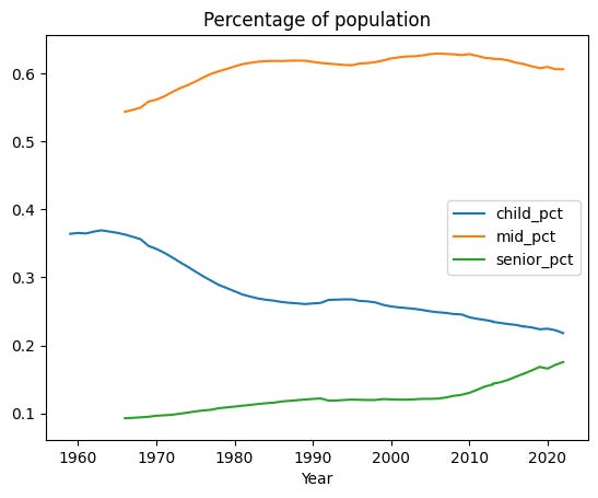
We can see from this that over years, the percentage of children in the overall population has declined, while the percentage of senior citizens and middle-aged people has risen.

Read values for the elderly (i.e., 65 and over) from the Excel file, where the ethnicity is listed as "Black alone" or "Black". (A handful of years will be duplicated; that's OK.)

Now let’s look at the data for Black Americans. On the one hand, creating this data frame involves a lot of repetition from what we did before. On the other hand, there are some special cases.

First, I created a basic data frame:

filename = 'tableA3_hist_pov_by_all_and_age.xlsx'

df = (
    pd.read_excel(filename,
                  header=[3,4,5],
                 na_values='N'                 )
    .iloc[209:270]
)

Notice that I used “iloc” to select particular rows. I knew which rows I wanted from the Excel file, but because I wanted two separate sections, I had to choose them a bit differently.

With that data in place, I decided that I only cared about the total population, and the percent (not number!) of people below the poverty line. I grabbed those as follows, renaming the columns to make them easier to work with:

df = df[df.columns[[0, -1]]]
df.columns=['raw_year', 'pct_black_poverty']

I then had to do the same kind of thing as before to turn the years into just four-digit years, without any potential problems with footnotes:

df = df.loc[     
    df['raw_year'].astype(str).str.isdigit() 
]

df['year'] = df['raw_year'].astype(str).str.slice(None, 4).astype(int) 

df = df.set_index('year').drop('raw_year', axis='columns')

The result? If we grab the only column in the data frame, we get a series showing the percentage of Black Americans under the poverty line:

BW 31: Poverty

First and foremost: Thanks to the many of you who sent warm, supportive messages in the wake of the unexpected passing of my father, Rabbi Barry Dov Lerner, two weeks ago. I learned much from my father, chief among them to love reading and learning -- and then to share what I had learned with others. My father came up with the name for Bamboo Weekly, and frequently gave me feedback and comments, even though he wasn't able to code.

You can read the eulogy I gave at the funeral at: https://docs.google.com/document/d/1PxSo9kGwIrkNK4FWatDEEWzXSP2R3OGdEn17eAeEZWU/edit?usp=sharing

And now, back to our regularly scheduled Pandas and data analysis.

While considering a topic to examine this week, I saw an article in the New York Times, "Poverty Rate Soared in 2022 as Aid Ended and Prices Rose" (https://www.nytimes.com/2023/09/12/business/economy/income-poverty-health-insurance.html?unlocked_article_code=NbtUcftR5hPRpr8EFtduQTWgqUzELOk4fBQind_8Kwd8ymQ4hN7-nmgINGD0JobiKZ0SE3NILUoooRkyWeHXvdXahh8XEEJzEFve71QqwwF-kSRFIwfNZp6XJnUB9i2oFsdhOxaalk20kEvksJyDsV3STWdDUXrK6o7Ge_YZP6AaCpZjbyj7BXTozhpCvhjIbNlcLav-niEA1vQXkyX1jVFBDHql_UORveyIRRIUu-QMefDRSVTpBHD59ImyUtUF4C0Ivgv0bJ7mDyJHBn0J2_ut5IyYd0Xsv7LYUgqJumY_E4XmXAJz6avYf8hCOA5W7MBFS0tA7701JpPAjyiA4Zt4K9UmWIOQgetdVyR2&smid=url-share). The article cited a report from the US Census Bureau indicating that while poverty levels in the US had declined in 2020 and 2021, they had risen in 2022. The Census Bureau's page describing the study is at https://www.census.gov/library/publications/2023/demo/p60-280.html , including a full report at /content/files/content/dam/Census/library/publications/2023/demo/p60-280.pdf .

Many countries measure poverty levels, and you might have heard mentions of these numbers in the news. But how exactly do you measure poverty? What amount of money is enough to put someone over the poverty line? Does that vary from place to place? What if the family receives government assistance — should that be included in the amount that the family receives, or not?

These and many other questions have led to the Census Bureau measuring poverty in two different ways. The original poverty measure (OPM) compares "pretax money income to a poverty threshold that is adjusted by family composition." That's fairly straightforward to compute, but it can miss a lot of factors that change whether a family should be considered poor. For that reason, the Census Bureau created the supplemental poverty measure (SPM), which includes government assistance, health expenses, and taxes. It's a newer measure, having started only in 2011, but the idea is that it more fully captures the nuances of poverty.

I was wondering what we can learn about poverty from the data. Have things really gotten better in the last few decades? Can we see the downturn in poverty from the last few years, followed by the uptick? Do we see differences in poverty rates for people of different ages and races? And while we're looking at census data, how many elderly vs. children live in the US, and how is that changing?

Data and eight questions

This week, we'll look at a small part of the data from the latest poverty survey, which was published just a few days ago. The overall download page is at:

https://www.census.gov/library/publications/2023/demo/p60-280.html

The data itself is broken up across several different Excel files. We'll only look at one of those files, whose download URL is:

/content/files/programs-surveys/demo/tables/p60/280/tablea3_hist_pov_by_all_and_age.xlsx

I have eight questions and tasks for you this week. The learning goals include working with Excel, cleaning data, grouping, plotting, and selecting rows and columns:

Read the "History POV by all and age" file into a data frame. We're only interested (for now) in the "ALL RACES" section. Turn the years into an index, and remove the "percent" measures.
In 2022, what was the number of Americans living below the poverty line?
Now calculate the percentage of all people below the poverty line in each year. In what year(s) was it highest and lowest?
For each year, calculate the percentage change in child poverty rate (i.e., for people under 18) from the previous year. In what five years did it rise the most? In what five years did it drop the most?
Calculate the mean percentage of child poverty per decade. How much more (or less) likely were children in the 1950s and 1960s to be poor than now?
For each year, what percentage of the population is under 18 years, 18-64 years, or 65+? Plot these percentages over time.
Read values for the elderly (i.e., 65 and over) from the Excel file, where the ethnicity is listed as "Black alone" or "Black". (A handful of years will be duplicated; that's OK.)
In 2022, what percentage of elderly Black people were defined as being in poverty? How does that compare with 1965, the first year for which we have data?

Selection deleted

import pandas as pd

# 1. Read the "History POV by all and age" file into a data frame. We're only interested

# (for now) in the "ALL RACES" section. Turn the years into an index, and remove the "percent" measures.

filename = '/Users/reuven/Downloads/tableA3_hist_pov_by_all_and_age.xlsx'

df = (

pd.read_excel(filename,

header=[3,4,5],

nrows=67,

na_values='N')

.drop(0)

.drop('Percent', axis='columns', level=2)

.assign(Year=lambda df_: df_[df_.columns[0]].astype(str).str.slice(None, 4).astype(int))

.set_index('Year')

)

Race, Hispanic origin, and year All people Under 18 years 18 to 64 years 65 years and over Unnamed: 0_level_1 Total Below poverty Total Below poverty Total Below poverty Total Below poverty Unnamed: 0_level_2 Unnamed: 1_level_2 Number Unnamed: 4_level_2 Number Unnamed: 7_level_2 Number Unnamed: 10_level_2 Number Year 2022 2022 330100.0 37920.0 71950.0 10780.0 200200.0 21240.0 57880.0 5897.0 2021 2021 328200.0 37930.0 72940.0 11150.0 199100.0 20980.0 56190.0 5802.0 2020 20201 327600.0 37550.0 73540.0 11790.0 199800.0 20910.0 54280.0 4852.0 2019 2019 324800.0 33980.0 72640.0 10470.0 197500.0 18660.0 54640.0 4858.0 2018 2018 323800.0 38150.0 73280.0 11870.0 197800.0 21130.0 52790.0 5146.0 ... ... ... ... ... ... ... ... ... ... 1963 1963 187300.0 36440.0 69180.0 16010.0 NaN NaN NaN NaN 1962 1962 184300.0 38630.0 67720.0 16960.0 NaN NaN NaN NaN 1961 1961 181300.0 39630.0 66120.0 16910.0 NaN NaN NaN NaN 1960 1960 179500.0 39850.0 65600.0 17630.0 NaN NaN NaN NaN 1959 1959 176600.0 39490.0 64320.0 17550.0 96690.0 16460.0 15560.0 5481.0

66 rows × 9 columns

df.columns = df.columns.droplevel(2)

df = df.drop(df.columns[0], axis='columns')

All people Under 18 years 18 to 64 years 65 years and over Total Below poverty Total Below poverty Total Below poverty Total Below poverty Year 2022 330100.0 37920.0 71950.0 10780.0 200200.0 21240.0 57880.0 5897.0 2021 328200.0 37930.0 72940.0 11150.0 199100.0 20980.0 56190.0 5802.0 2020 327600.0 37550.0 73540.0 11790.0 199800.0 20910.0 54280.0 4852.0 2019 324800.0 33980.0 72640.0 10470.0 197500.0 18660.0 54640.0 4858.0 2018 323800.0 38150.0 73280.0 11870.0 197800.0 21130.0 52790.0 5146.0 ... ... ... ... ... ... ... ... ... 1963 187300.0 36440.0 69180.0 16010.0 NaN NaN NaN NaN 1962 184300.0 38630.0 67720.0 16960.0 NaN NaN NaN NaN 1961 181300.0 39630.0 66120.0 16910.0 NaN NaN NaN NaN 1960 179500.0 39850.0 65600.0 17630.0 NaN NaN NaN NaN 1959 176600.0 39490.0 64320.0 17550.0 96690.0 16460.0 15560.0 5481.0

66 rows × 8 columns

df.loc[

2022,

('All people', 'Below poverty')

]

37920.0

# 2. In 2022, what was the number of Americans living below the poverty line?

df.loc[

2022,

('All people', 'Below poverty')

] * 1000

# 3. Now calculate the percentage of all people below the poverty line in each year.

# In what year(s) was it highest and lowest?

(df[('All people', 'Below poverty')] / df[('All people', 'Total')]).agg(['idxmax', 'idxmin'])

idxmax    1959
idxmin    2019
dtype: int64

# 4. For each year, calculate the percentage change in child poverty rate

# (i.e., for people under 18) from the previous year. In what five years did it rise

# the most? In what five years did it drop the most?

(

(df[('Under 18 years', 'Below poverty')] / df[('Under 18 years', 'Total')])

.pct_change(periods=-1)

.sort_values(ascending=False)

.head(5)

)

Year
1980    0.120059
2020    0.112293
1975    0.110146
1982    0.092877
1981    0.092040
dtype: float64

(

(df[('Under 18 years', 'Below poverty')] / df[('Under 18 years', 'Total')])

.pct_change(periods=-1)

.sort_values(ascending=True)

.head(5)

)

Year
1966   -0.158759
2019   -0.110173
1969   -0.098325
1999   -0.092795
1965   -0.089017
dtype: float64

Selection deleted

# 5. Calculate the mean percentage of child poverty per decade. How much

# more (or less) likely were children in the 1950s and 1960s to be poor than now?

(

df['Under 18 years']

.assign(decade=lambda df_:df_.index//10*10,

pct=lambda df_:df_['Below poverty']/df_['Total'])

.groupby('decade')['pct'].mean()

.sort_values(ascending=False)

)

decade
1950    0.272854
1960    0.208422
1990    0.206398
1980    0.204687
2010    0.192852
2000    0.177277
1970    0.157030
2020    0.154338
Name: pct, dtype: float64

<pandas.core.groupby.generic.DataFrameGroupBy object at 0x130753650>

# 6. For each year, what percentage of the population is under 18 years, 18-64 years,

# or 65+? Plot these percentages over time.

(

df.xs('Total', level=1, axis='columns')

.assign(child_pct=lambda df_:df_['Under 18 years'] / df_['All people'],

mid_pct=lambda df_:df_['18 to 64 years'] / df_['All people'],

senior_pct=lambda df_:df_['65 years and over'] / df_['All people'],

)

.filter(like='pct', axis='columns')

.plot.line(title='Percentage of population')

)

<Axes: title={'center': 'Percentage of population'}, xlabel='Year'>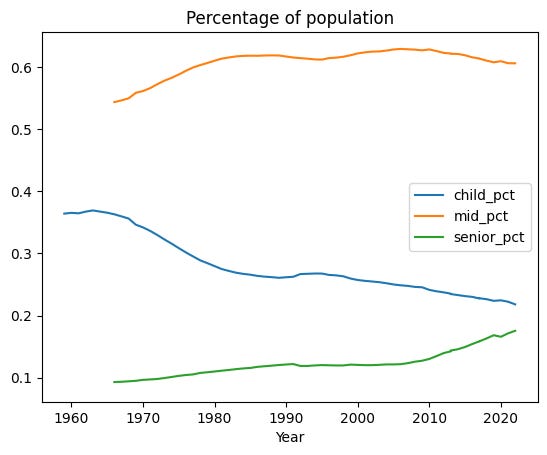

# 7. Read values for the elderly (i.e., 65 and over) from the Excel file,

# where the ethnicity is listed as "Black alone" or "Black". (A handful of

# years will be duplicated; that's OK.)

filename = '/Users/reuven/Downloads/tableA3_hist_pov_by_all_and_age.xlsx'

df = (

pd.read_excel(filename,

header=[3,4,5],

na_values='N' )

.iloc[209:270]

)

df = df[df.columns[[0, -1]]]

df.columns=['raw_year', 'pct_black_poverty']

df = df.loc[

df['raw_year'].astype(str).str.isdigit()

]

df['year'] = df['raw_year'].astype(str).str.slice(None, 4).astype(int)

df = df.set_index('year').drop('raw_year', axis='columns')

df['pct_black_poverty']

year
2022    17.6
2021    17.8
2020    17.2
2019    18.0
2018    18.9
2017    19.0
2017    19.3
2016    18.7
2015    18.4
2014    19.2
2013    18.7
2013    17.6
2012    18.2
2011    17.3
2010    17.9
2009    19.5
2008    20.0
2007    23.2
2006    22.7
2005    23.3
2004    23.8
2003    23.7
2002    23.8
2001    21.9
2000    21.8
1999    22.8
1998    26.4
1997    26.0
1996    25.3
1995    25.4
1994    27.4
1993    28.0
1992    33.5
1991    33.8
1990    33.8
1989    30.7
1988    32.2
1987    32.4
1986    31.0
1985    31.5
1984    31.7
1983    36.0
1982    38.2
1981    39.0
1980    38.1
1979    36.2
1978    33.9
1977    36.3
1976    34.8
1975    36.3
1974    34.3
1973    37.1
1972    39.9
1971    39.3
1970    48.0
1969    50.2
1968    47.7
1967    53.3
1966    55.1
1965    62.5
Name: pct_black_poverty, dtype: float64

In 2022, what percentage of elderly Black people were defined as being in poverty? How does that compare with 1965, the first year for which we have data?

That’s a lot of data! If we just want 2022 (the most recent year for which we have data) and 1965 (the first year for which we have data), we can use the two-argument version of “loc”:

df.loc[[2022, 1965], 'pct_black_poverty']

The result:

year
2022    17.6
1965    62.5
Name: pct_black_poverty, dtype: float64

The bad news? In 2022, 17.6 percent of Black Americans were under the poverty line. That’s quite a bit higher than the overall population, at 11.5 percent.

The good news? Back in 1965, 62.5 percent (!) of Black Americans were under the poverty line. That is … an astonishing number, and points to improvement, if slow and still insufficient.

And that’s it for this week! Questions, comments, or suggestions? Share them with everyone.

My Jupyter notebook can be downloaded from here: https://drive.google.com/file/d/17OnaLPhr-ho2YObcXW0xVgUIl2jHfbql/view?usp=sharing

I’ll be back next Wednesday with another set of problems based on current events.

Until then,

Reuven

Bamboo Weekly #31: Poverty (solutions)

Data and eight questions

Read the "History POV by all and age" file into a data frame. We're only interested (for now) in the "ALL RACES" section. Turn the years into an index, and remove the "percent" measures.

In 2022, what was the number of Americans living below the poverty line?

Now calculate the percentage of all people below the poverty line in each year. In what year(s) was it highest and lowest?

For each year, calculate the percentage change in child poverty rate (i.e., for people under 18) from the previous year. In what five years did it rise the most? In what five years did it drop the most?

Calculate the mean percentage of child poverty per decade. How much more (or less) likely were children in the 1950s and 1960s to be poor than now?

For each year, what percentage of the population is under 18 years, 18-64 years, or 65+? Plot these percentages over time.

Read values for the elderly (i.e., 65 and over) from the Excel file, where the ethnicity is listed as "Black alone" or "Black". (A handful of years will be duplicated; that's OK.)

BW 31: Poverty

Data and eight questions

In 2022, what percentage of elderly Black people were defined as being in poverty? How does that compare with 1965, the first year for which we have data?

Bamboo Weekly #31: Poverty

Bamboo Weekly #32: Unions

Bamboo Weekly #31: Poverty (solutions)

Data and eight questions

Read the "History POV by all and age" file into a data frame. We're only interested (for now) in the "ALL RACES" section. Turn the years into an index, and remove the "percent" measures.

In 2022, what was the number of Americans living below the poverty line?

Now calculate the percentage of all people below the poverty line in each year. In what year(s) was it highest and lowest?

For each year, calculate the percentage change in child poverty rate (i.e., for people under 18) from the previous year. In what five years did it rise the most? In what five years did it drop the most?

Calculate the mean percentage of child poverty per decade. How much more (or less) likely were children in the 1950s and 1960s to be poor than now?

For each year, what percentage of the population is under 18 years, 18-64 years, or 65+? Plot these percentages over time.

Read values for the elderly (i.e., 65 and over) from the Excel file, where the ethnicity is listed as "Black alone" or "Black". (A handful of years will be duplicated; that's OK.)

BW 31: Poverty

Data and eight questions

In 2022, what percentage of elderly Black people were defined as being in poverty? How does that compare with 1965, the first year for which we have data?

Read next

Bamboo Weekly #31: Poverty

Bamboo Weekly #32: Unions