


This week, we looked at high-temperature data, in an attempt to see where and when it has been particularly hot over the years, and whether we can see a general trend toward hotter temperatures.
Our data this week came from the National Centers for Environmental Information (NCEI), part of the National Oceanic and Atmospheric Administration (NOAA), part of the US Department of Commerce.
The data is huge, even after we whittle it down and use only a part of it. Part of this week’s learning goals to include taking a large number of files and turning them into a data frame containing only some of the data.
I first suggested that you look through the data dictionary for this data set, to understand the structure and contents of what we’re going to be working with. The data dictionary is located here:
https://www.ncei.noaa.gov/pub/data/ghcn/daily/readme.txt
I then gave you 7 questions and tasks for this week, the bulk of the work being in question 3, where we create the data frame based on the files.
So, without further ado, let’s get to this week’s questions:
Download the list of weather stations (https://www.ncei.noaa.gov/pub/data/ghcn/daily/ghcnd-stations.txt) and turn it into a data frame. Use the specifications for the file, as described in the README. You'll want to set your own names for the column headers. Make the `id` column into the index.
There are a lot of weather stations positioned all over the world, and the data set that we’re working with this week includes data from all of them. Each weather station has a unique ID, as well as a location name, longitude, and latitude. Turning the stations into a data frame is a good first step.
Before doing anything else, I decided to load up NumPy and Pandas:
import numpy as np
import pandas as pd
from pandas import Series, DataFrame
With those in place, I then started to work on the data itself, create a new data frame with the station information.
Most of the time, we deal with files in CSV or Excel format. However, the stations aren’t in either of those formats, as you might have seen in the data dictionary. Instead, they are in “fixed-width format,” meaning that while each line in the file contains a single record, the fields aren’t separated by delimiter characters. Rather, each field contains a specific number of characters.
Fortunately, Pandas comes with read_fwf, a method for reading from fixed-width field files. If you read through the README file, you’ll see that section IV indicates that each line contains 85 characters, divided into nine fields:
------------------------------
Variable   Columns   Type
------------------------------
ID            1-11   Character
LATITUDE     13-20   Real
LONGITUDE    22-30   Real
ELEVATION    32-37   Real
STATE        39-40   Character
NAME         42-71   Character
GSN FLAG     73-75   Character
HCN/CRN FLAG 77-79   Character
WMO ID       81-85   Character
------------------------------
In theory, we could call read_fwf without any arguments other than the filename from which we want to read. But in reality, that’ll give us a huge mess. That’s because by default, read_fwf tries to infer where the columns are. In a file like this one, where there are numerous empty fields, it’ll quickly get confused and give us the wrong number of fields.
Fortunately, the data dictionary tells us the columns used by each field. Which means that we can indicate which field goes where by passing a list of tuples to the “colspecs” argument:
stations_df = pd.read_fwf(stations_filename,
                 colspecs=[(0,11), (12, 20), (21,30), (31,37), (38,40), (41,71), (72, 75), (76,79), (80,85)])
First of all, notice that the numbers in my tuples and the numbers in the above specification from the README aren’t quite the same. That’s because the data dictionary called the first column 1 — but in Python, the first column is 0. We thus need to subtract 1 from the starting point for each of the columns.
What about the ending point? Shouldn’t the first tuple be (0, 10) rather than the specified (1, 11)? No, because Python (and read_fwf) almost always assume “up to but not including” the endpoint. So when we say (0, 11), we mean that we want 11 characters, starting with index 0, and going through index 10.
I’m not sure why, but the format used for the stations leaves an empty character between columns, which just makes it more confusing.
If you use the above code to read in the file, you’ll quickly discover that it’s still a bit weird. That’s because read_fwf, like read_csv, assumes that the first row names the columns. To convince it otherwise, we’ll need to set “header=None”, indicating that there are no headers in this file, and then pass a list of strings to the “names” argument, telling it what to call the columns.
Finally, we can pass “index_col” and name the “id” column (defined in “names” above) as our index:
stations_df = pd.read_fwf(stations_filename,
                 header=None,
                 names='id latitude longitude elevation state name gsn_flag hcn_crn_flag wmo_id'.split(),
                 colspecs=[(0,11), (12, 20), (21,30), (31,37), (38,40), (41,71), (72, 75), (76,79), (80,85)] ,
                 index_col='id')
The result is a data frame with 124,954 rows, each describing a different weather-monitoring station somewhere in the world.
Download the GHCND-ALL data (https://www.ncei.noaa.gov/pub/data/ghcn/daily/ghcnd_all.tar.gz). NOTE: This file is 3.4 GB in size, so it might take a while to download to your computer. Follow the directions in the README to un-tar the file. This will result in about 30 GB of files being created under the `ghcnd_all` directory.
Most people are used to working with zipfiles. A zipfile can contain a number of files within it, and also compresses those files. It’s thus super convenient to work with zip.
But before zip came along, there was “tar” format, short for “tape archive.” The idea of a tarfile was that you could take a whole bunch of files and put them together inside of one file, typically for backup purposes. I could “tar up” an entire directory, including its files and subdirectories, and store that file somewhere. Then, if/when I need to retrieve those files, I could untar them.
Note that tar archived files, but didn’t compress them. A few different compression schemes existed at the time, but the “GNU zip” format (aka “gzip”), from the people at the Free Software Foundation (sort of a predecessor to the open-source movement), quickly took hold. Note that there was no connection between gzip and the zip that we now know; I’d argue that this was a foolish choice on the GNU people’s part, but there you have it.
In the Unix world, it’s thus pretty common to have a file with the “.tar.gz” dual suffix. To open the file, you first need to un-gzip it, and then you have to un-tar it. There are far too many options to both tar and gzip to explain them here, but the README explains that after you have downloaded the ghcnd_all.tar.gz file, you can open it up into a directory with the following command:
tar xzvf ghcnd_all.tar.gzIn short, the above command first un-gzips the file (that’s the “z” option), then extracts the file (that’s the “x” option), doing it verbosely (i.e., telling us what it’s doing) and working on the file we specify (i.e., ghcnd_all.tar.gz).
The gzipped tarfile that we downloaded is 3.4 GB in size. And when opened up, into a new directory? The complete contents are 30 GB, with 124,946 files, each ending with “.dly”, meaning that it contains daily information from a particular weather station.
Create a data frame with just the TMAX readings, from all stations starting in 1990. Only store the station ID, year, month, date, and the reading value.
This part of things was … challenging, for at least two reasons: First, there were a lot of files, adding up to a large amount of data. Second, we needed to transform the data from each of the “dly” files into something that could be used as a data frame.
I decided to do this in three stages:
- First, I would iterate over every line, of every file, keeping only those lines with a maximum-temperature reading (i.e., TMAX). The result would be a list of strings.
- Then, I would iterate over that list of strings, filtering out the records that we don’t want or need, and returning a dict for each record that we do keep.
- Create a data frame based on the list of dicts.
So, let’s step through this, one piece at a time.
First: Each of the 124,946 “.dly” files has a common format:
Each file is from a single weather station. The filename (without the extension) is the weather station’s code, now the index in “stations_df”.
Each line in a file contains the measurements of one weather statistic for one month. If we have 12 months and 10 statistics, then there will be 120 lines in the file.
As indicated in the README, these files (like the station file) use fixed-width fields. The first field contains:
the station ID
the 4-digit year
the 2-digit month
a four-character code indicating what measurement we’re taking
For example, here’s the first field from one file:
ACW00011604194901TMAXThis is from weather station ACW00011604, January 1949, measuring max temperature.
Then, for each day of the month, there will be four pieces of additional information:
- The measured value
- Measurement flag (when was it measured?)
- Were there quality problems?
- What is the source?
We’re going to ignore all but the first value.
For each of the 31 potential days in a month, all four of these appear; each line will contain exactly 269 characters.
Missing data is indicated by having a value of -9999.
So, how can I create a list of strings based on the TMAX lines in every “.dly” file in this directory? I decided to use a nested list comprehension, iterating over every line in every file that I can find with the standard library’s “glob” module:
import glob

all_tmax = [one_line.removesuffix('\n')
 for one_filename in glob.glob('ghcnd_all/*.dly')
 for one_line in open(one_filename)
 if one_line.split()[0].endswith('TMAX')
 if int(one_line[11:15]) > 1990]]
What does this do? Let’s take it apart, bit by bit:
- I use glob.glob to return a list of all files matching the pattern “ghcnd_all/*.dly”, or the daily files.
- I then iterate over each of the filenames in that list, assigning each filename in turn to the variable one_filename.
- I then go through each of the files, one line at a time, assigning each line to the variable “one_line”.
- I split the line on whitespace, checking whether the first element of that list ends with the string TMAX.
- I also grab the year from the string, and check whether it’s greater than 1990.
- If both of these conditions are true (i.e., if it’s a TMAX reading from after 1990), we add the string (minus its newline) to the output.
When we’re done with this process, we have a list of 5,944,767 269-character strings. Each string represents one month’s max temperature readings from one weather station.
Here’s what all_tmax[:3] looks like on my computer:
['AM000037959199004TMAX   72  S-9999      60  S-9999   -9999   -9999   -9999     181  S-9999   -9999   -9999   -9999     205  S  200  S  126  S-9999   -9999   -9999   -9999     220  S  141  S-9999     209  S  212  S  210  S-9999     266  S-9999     189  S-9999   -9999   ',
 'AM000037959199006TMAX  312  S-9999     336  S-9999   -9999   -9999     282  S  322  S-9999   -9999   -9999     310  S  322  S-9999   -9999     232  S-9999     238  S-9999     205  S  250  S-9999   -9999     303  S  285  S-9999   -9999   -9999   -9999     248  S-9999   ',
 'AM000037959199011TMAX  202  S-9999   -9999   -9999   -9999     255  S-9999     150  S-9999     125  S-9999   -9999     104  S-9999   -9999     122  S-9999     180  S  202  S-9999     180  S  174  S-9999   -9999   -9999   -9999   -9999   -9999     188  S-9999   -9999   ']
Next, I want to turn this list of strings into a list of dicts. It would almost certainly use less memory to use a list of lists, but I find dicts easier to think about and work with, and decided that the memory hit wouldn’t be too bad.
I decided to perform this transformation using a standard “for” loop, appending to a list. I could also have done it using a combination of a function and a list comprehension — and yes, I could have done it in a single pass with the above list comprehension and a function — but I often prefer to do things in stages, so that I can see what’s happening and debug it.
(For example, an earlier version of the above code used “strip” to remove the newline at the end. That had the side effect of removing trailing spaces. I also decided to use a second “if” statement in the above list comprehension to filter by year, rather than doing it in my dict-building “for” loop. By splitting things into pieces, I was able to debug, refactor, and try different approaches.)
Here’s the code I came up with to create a list of dicts with all records for my data frame:
all_records = []

for index, one_record in enumerate(all_tmax):
    if index % 1_000_000 == 0:
        print(f'{index:12,} -- ({(index/len(all_tmax)) * 100:2.2f}% done)')
    station_id = one_record[:11]
    year = int(one_record[11:15])
    month = int(one_record[15:17])
    element = one_record[17:21]

    for day_number, day_start in enumerate(range(21,269,8), 1):
        value = one_record[day_start:day_start+5]

        if value and float(value) == -9999:
            continue   # ignore NaN values

        measurement_flag = one_record[day_start+5:day_start+6]
        quality_flag = one_record[day_start+6:day_start+7]
        source_flag = one_record[day_start+7:day_start+8]

        all_records.append(
             {'station_id':station_id,
              'year':year,
              'month':month,
              'day':day_number,
              'value':float(value) / 10})  # tenths of degrees Celsius

print('Done')
So, what’s happening here? Truth be told, not that much: We’re iterating over a list of strings, grabbing slices from each of those strings, and then turning them into a dict with specified keys and values.
The tricky thing is that each row of the file represents 31 different readings, one for each day in the month. Yes, even months without 31 days have 31 entries, with values of -9999 to indicate NaN. The value -9999 is also used to indicate that there was a problematic or missing reading. In all of these cases, we’ll just ignore values of -9999.
We’ll also ignore the measurement, quality, and source flags; if you have enough time and memory to include them in your data frame, then that’s great, and you can do tons of sophisticated analysis on max temperatures. But since we aren’t going to use them, I left them out of the output dict.
Notice that I used “enumerate” in two places:
- In the outer “for” loop, iterating over the strings in “all_tmax”. This was just so that I could get a printout indicating how far along we were in processing the data. I often like to use this sort of loop and printout when I’m nervous about how long things are taking. I took advantage of the formatting we can do in f-strings to display the number of records we have processed, as well as the percentage we have finished, in a nice way. If you’re curious about f-string formatting, take a look at the handy guide at https://fstring.help/.
- In the inner “for” loop, iterating over the indexes in the current string. Each day’s entry consumes 8 characters, and I used “enumerate” to count which day of the month we’re on. I passed a second, optional argument to “enumerate” so that it would start counting days with 1, not 0.
And yes, I used “range” to get the start of the fields for each day of the month, starting with character 21 and going up to the end of the string, adding 8 with each iteration.
I ended up with a list of 174,668,969 dictionaries, each representing one TMAX reading from one day at one weather station.
This is what I get from requesting all_records[:3]:
[{'station_id': 'AM000037959',
  'year': 1990,
  'month': 4,
  'day': 1,
  'value': 7.2},
 {'station_id': 'AM000037959',
  'year': 1990,
  'month': 4,
  'day': 3,
  'value': 6.0},
 {'station_id': 'AM000037959',
  'year': 1990,
  'month': 4,
  'day': 8,
  'value': 18.1}]
Notice that the temperature is measured in degrees Celsius. In my “for” loop, I took the value in the file and divided it by 10, since the README indicated that the stored values were in tenths of degrees Celsius.
With this list of dicts in place, I can now create a data frame:
df = DataFrame(all_records)I know, this code is a bit of a let-down, after everything we’ve written before. But it works, and it works well!
I should note that each of these steps took a long time to run, even on my souped-up iMac with tons of RAM. (I’m told that Apple’s newer M1 and M2 chips run far faster than my machine, but I’m guessing that it’ll still take a while.)
How much memory is the data currently using? Can you cut that down?
If we want to know how much memory a data frame is using, we can use the memory_usage method on our data frame:
Index                132
station_id    1397351752
year          1397351752
month         1397351752
day           1397351752
value         1397351752
dtype: int64
This doesn’t mean much on its own, but because we got a series back, we can invoke “sum” on the numbers and get a total of 6,986,758,892. In other words, our data frame is using 6.9 GB.
We can get a similar reading if we use the “info” method, which summarizes everything about a data frame:
<class 'pandas.core.frame.DataFrame'>
RangeIndex: 174668969 entries, 0 to 174668968
Data columns (total 5 columns):
 #   Column      Dtype
---  ------      -----
 0   station_id  object
 1   year        int64
 2   month       int64
 3   day         int64
 4   value       float64
dtypes: float64(1), int64(3), object(1)
memory usage: 6.5+ GB
See the final line there, where it says how much memory we’re using? It says 6.5+ GB. What is the + doing there?
The thing is, Pandas isn’t really calculating all of the memory we’re using. Rather, it’s calculating the memory being used by the NumPy backend. That includes all of the numeric values, but it doesn’t include the strings — which are what we’re using for the “station_id” column.
We can force Pandas to perform a real check, and calculate the lengths of the strings we’re using, by passing the memory_usage='deep' keyword argument to info. This takes far longer to execute, but gives us a truly accurate count of how much memory is being used. The result:
<class 'pandas.core.frame.DataFrame'>
RangeIndex: 174668969 entries, 0 to 174668968
Data columns (total 5 columns):
 #   Column      Dtype
---  ------      -----
 0   station_id  object
 1   year        int64
 2   month       int64
 3   day         int64
 4   value       float64
dtypes: float64(1), int64(3), object(1)
memory usage: 16.3 GB
See that? We’re actually using 16.3 GB of RAM. Which is indeed more than 6.5 GB, but … that first number was off by quite a bit.
How can we pare that memory usage down? By changing the dtypes we’re using to smaller values. (I’m guessing that we could also save memory by using PyArrow, but I decided not to overcomplicate things here.) Consider:
- We cannot really change the strings used by station_id. We’re stuck with those, unless we switch to PyArrow.
- The year is an integer, but doesn’t need 64 bits. We can’t use 8 bits (since that’ll max out at 256), but we can definitely use 16.
- The month and day can both be 8-bit integers.
- The value can be a 16-bit float; we only care about tenths of degrees, anyway. (You could also argue that we could keep these values as integers, stored with their original values, and then use 8-bit integers for even bigger memory savings.)
Let’s change the dtypes of these columns:
df['year'] = df['year'].astype(np.int16)
df['month'] = df['month'].astype(np.int8)
df['day'] = df['day'].astype(np.int8)
df['value'] = df['value'].astype(np.float16)
How much memory are we using now?
<class 'pandas.core.frame.DataFrame'>
RangeIndex: 174668969 entries, 0 to 174668968
Data columns (total 5 columns):
 #   Column      Dtype
---  ------      -----
 0   station_id  object
 1   year        int16
 2   month       int8
 3   day         int8
 4   value       float16
dtypes: float16(1), int16(1), int8(2), object(1)
memory usage: 12.0 GB
In other words, we’ve saved more than 4 GB of memory, with no reduction in the accuracy of our data, with just a few short commands. This is still a relatively large data set, but it’s far more manageable than would otherwise have been the case.
What were the 20 highest temperatures ever recorded? What were the names of the weather stations where they were recorded?
Now that we have our data in place, we can start to conduct actual queries. First off, what were the 20 highest temperatures ever recorded? To find that, we’ll sort our data by the “value” columns, highest to lowest, and grab the top 20 rows with “head”:
df.sort_values('value', ascending=False).head(20)This works just fine, but it gives us the IDs of the weather stations where those measurements were taken, not their names. Those names are back in the “stations_df” data frame we started with. However, we can set the station ID to be the index of our data frame, and then join it with stations_df, thus getting the names:
(
    df.sort_values('value', ascending=False)
    .head(20)
    .set_index('station_id')
    .join(stations_df)
)
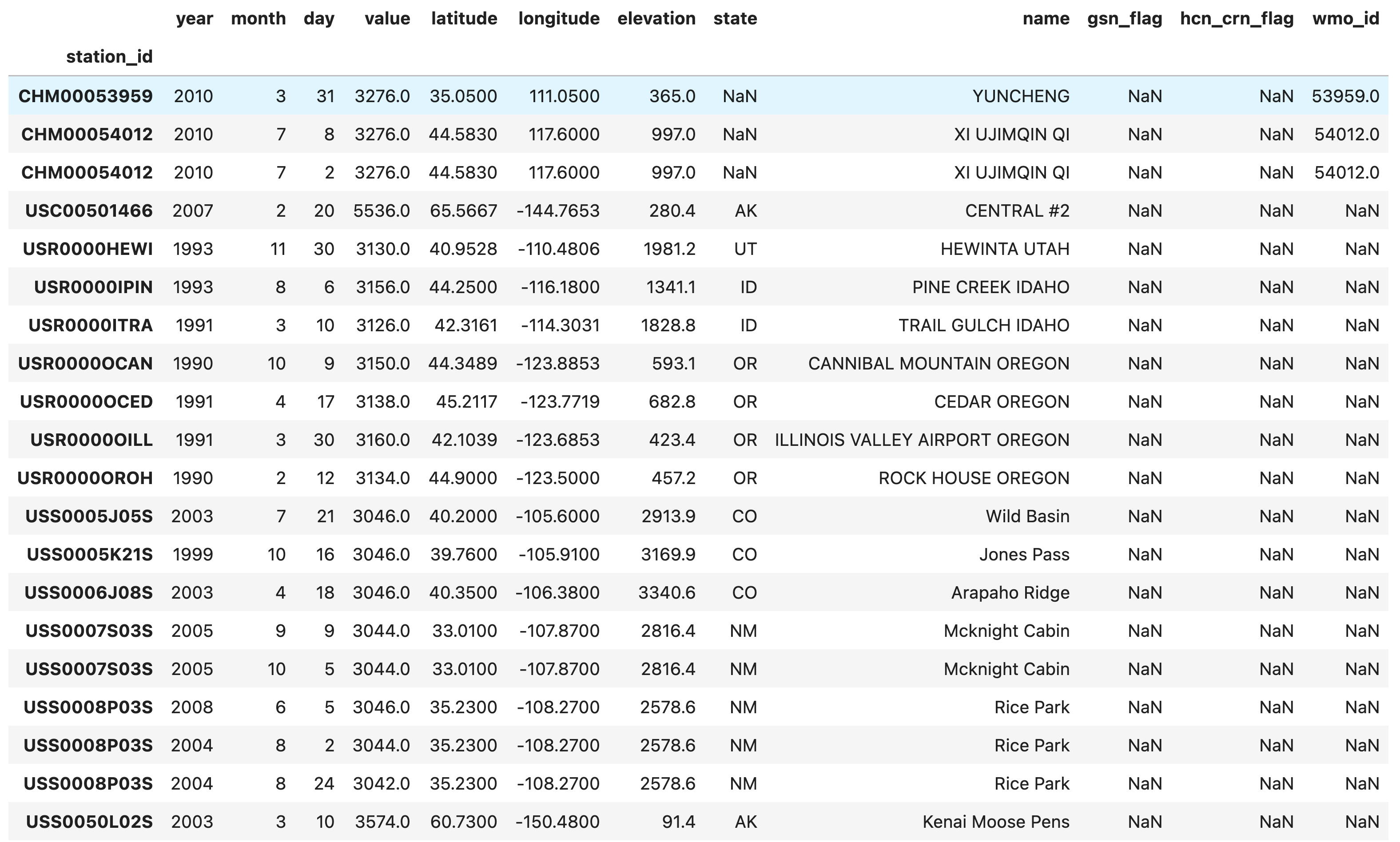
Sure enough, I get all of the information I wanted:
(And yes, it did occur to me that with the longitude and latitude, we could use GeoPandas to put this data on a map… but this is a weekly set of exercises, not a weekly book, so I had to put that thought aside.)
We can see that the three highest temperatures were outside of the United States (since the “state” column is NaN), and all (from the names) appear to be in China. I was surprised to see Alaska named as having a particularly high temperature. And indeed, all of these temperatures are suspiciously high. I’m wondering whether I messed up in my interpretation of the data (definitely possible!) or if the data was input in the wrong way. Or both. The fact that the temperatures are numbers like 3276 tells me that perhaps they should have been seen as 32.76 Celsius, a not-unreasonable reading — but not what I saw in the README.
I actually went back, after seeing these results, and added the quality flag to my data frame. I wanted to know if there was some consistently wrong or weird thing that I was missing. Sure enough, all of these values had a quality code of X, “failed bounds check.” So… the data was wrong, and as marked as such. And I guess I shouldn’t have told you to ignore the quality score!
Indeed, I found that 808,945 rows in our data frame had a quality code that wasn’t a single space character (i.e., had problems). I removed those rows:
df = df.loc[df['qflag'] == ' ']Then I re-ran my query:
(
    df.sort_values('value', ascending=False)
    .head(20)
    .set_index('station_id')
    .join(stations_df)
)
The result seems much more reasonable now:
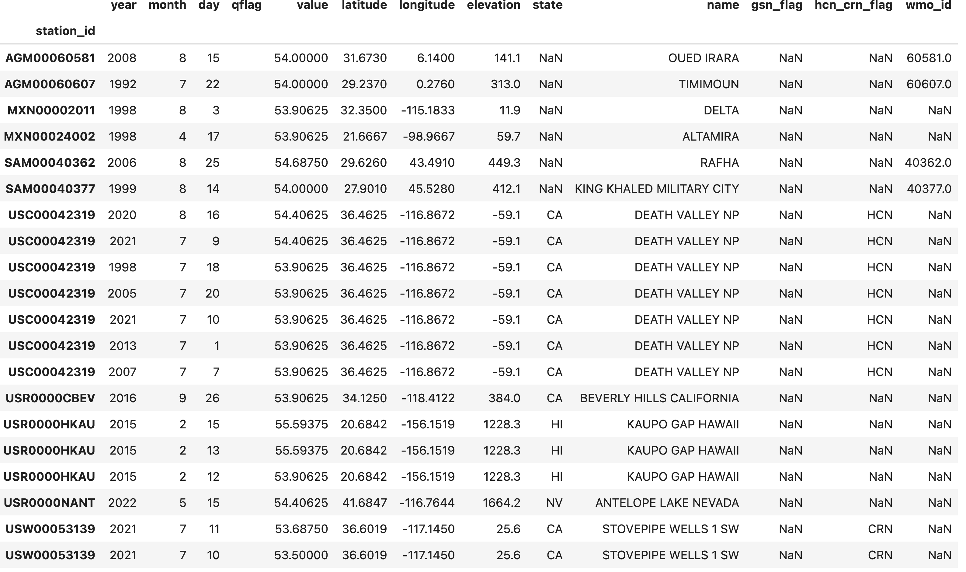
I hadn’t heard of some of these places (e.g, Oued Irara is in Algeria, for example), but several are in places (Saudi Arabia and California) that are known to be super hot.
I’m not sure if all of the data is 100 percent reliable; when you hear that people in Beverly Hills are hot, temperature isn’t usually what you think about. But this definitely seems more reliable and in line with my expectations than the previous data.
What 10 weather stations have, on average, had the highest recorded temperatures?
With the cleaned-up data in place, let’s now find out which weather stations have, on average, recorded the highest temperatures. First, my code:
(
    df.groupby('station_id')
    [['value']]
    .mean()
    .sort_values('value', ascending=False)
    .head(10)
    .join(stations_df)
)
In the above code, I first run a “groupby”, so that I’ll get one result per value of station_id. The result will be from running “mean” on the “value” column — meaning, we’ll get the mean temperature recorded at each station.
Notice that I used [['value']] here. I could have used just ['value'], but that would have returned a series, and I wanted to join the result with a data frame — and a series doesn’t have the “join” method. I thus got a data frame back (by asking for the results on a list of columns, even though that list had a single element), sorted it by value, got the 10 highest-value rows, and then joined it with stations_df:
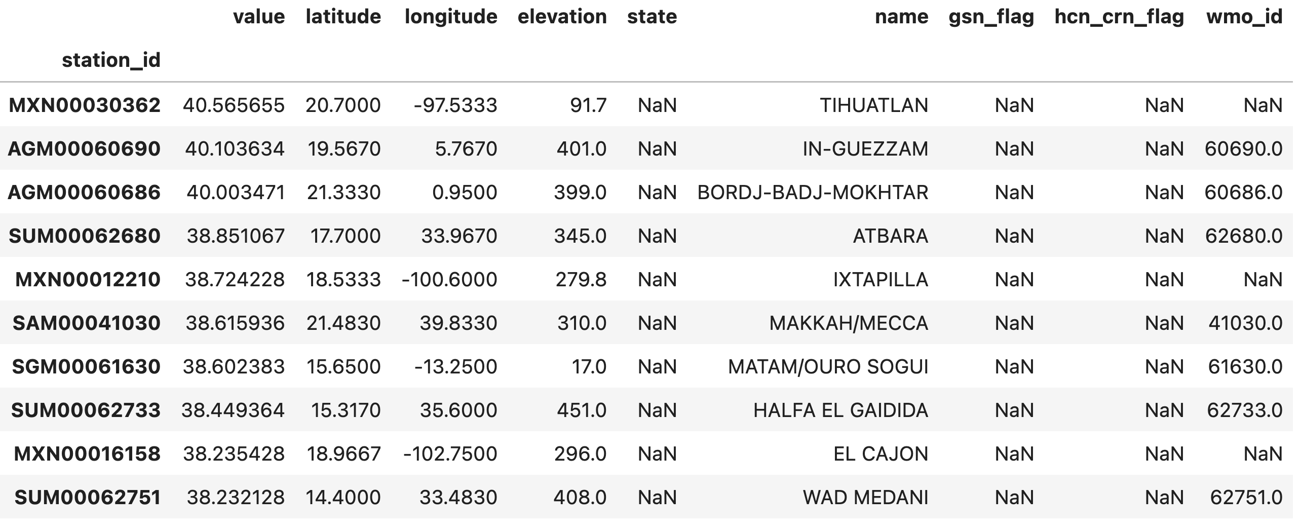
On average, then, the highest max temperatures are in Tihuatlan (Mexico) and In-Guezzam (Algeria).
Plot the average global temperature for each month over the last 10 years. Do we see the values rising?
Finally, I asked you to plot average global temperatures for each month over the last 10 years.
First, we’ll need to calculate the mean high temp for each month. We can do that with “groupby”, grouping on both “year” and “month”, then using the “plot” method:
df.groupby(['year', 'month'])['value'].mean().plot.line()This produces the following plot:

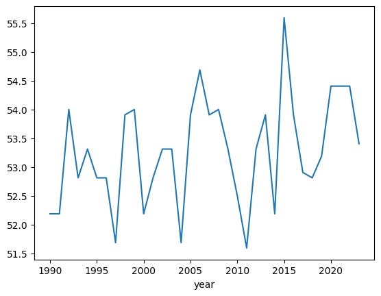
I don’t see much of a clear trend in the mean temperatures. But perhaps that’s the wrong measure; instead of looking at monthly averages, I can look at the annual maximums:
df.groupby('year')['value'].max().plot.line()I don’t know about you, but I definitely see a trend that’s generally moving up and to the right here:
Whew! I’ve often heard people say that 80% of data science involves cleaning the data before you even start to do the analysis. As we saw this week, that’s definitely the case. Moreover, even after you’ve started, you often need to double back and make corrections.
Questions? Comments? Suggestions? Share them with me, and others!
Meanwhile, my Jupyter notebook for this week is here: https://drive.google.com/file/d/17_44B6aiSdaAD1hk8ZEdR-aPlK9XdwN_/view?usp=sharing
I’ll be back on Wednesday with another problem from current events.
Reuven