


Last week, about $6 billion in bitcoin was stolen from Binance, one of the world's largest cryptocurrency exchanges, which seems to be the largest-ever heist of crypto. Experts are pointing to North Korea as the culprit, according to reports on the Slate Money podcast (https://slate.com/podcasts/slate-money/2026/10/artificial-intelligence-anthropic-wall-street-stock-market-ipo-bitcoin-heist-binance) and in the New York Times (https://www.nytimes.com/2026/10/30/business/binance-hack-crypto-price-what.html?unlocked_article_code=1.N1E.CRBJ.CCbv-ldQ_zXw&smid=url-share).
This week, we looked at the history of crypto heists. We'll see who was hacked, how much the heists were worth, how much money was returned, and whether such crimes are increasing over time.
Along the way, we'll explore some of the new functionality that was included in Pandas 3.1, which was released on October 22nd (https://pandas.pydata.org/docs/dev/whatsnew/v3.1.0.html).
Data and five questions
This week's data comes from DeFiLlama (https://defillama.com/), a crypto analytics site. They provide a free API at https://api.llama.fi/hacks, which returns JSON data about famous (and known) crypto heists. This will be our data set for this week.
Paid subscribers, both to Bamboo Weekly and to my LernerPython+data membership program (https://LernerPython.com) get all of the questions and answers, as well as downloadable data files, downloadable versions of my notebooks, one-click access to my notebooks, and invitations to monthly office hours.
Learning goals for this week include: Retrieving from APIs, working with JSON data, dates and times, grouping, plotting with Plotly, and new Pandas 3.1 functionality.
Here are my solutions and explanations for this week's questions:
Retrieve the data from DeFiLllama's API, and turn it into a Pandas data frame in which date is the index. Create a line plot showing, for each year, how many hacks were reported. Do we see a trend?
I started off by importing Pandas and Plotly Express. I thought that I was going to need to import requests as well, in order to retrieve the JSON data from the DeFiLlama API, but then I remembered that read_json, like all of the read_ methods in Pandas, can take a URL, not just a filename. Not all JSON is formatted in a way that read_json can use it, but it was in this case.
After creating the data frame, I then invoked set_index to turn the date column into the data frame's index, and then sort_index so that it would be sorted chronologically. The first is needed because read_json doesn't have an index_col keyword argument (which is in both read_csv and read_excel). And I sorted based on the index so that retrieving by date will work more consistently:
hacks_url = 'https://api.llama.fi/hacks'
df = (
    pd
    .read_json(hacks_url)
    .set_index('date')
    .sort_index()
)
The resulting data frame has 1,337 rows and 13 columns.
Normally, counting the number of hacks per year would involve a groupby on the year. But because the index contains datetime values, we can use a related method, namely resample, invoking count on the name column (although we could use any without NaN values). I set the time specifier to '1YE', meaning 1-year intervals, measured at the end. That gave, for each year in the data set, the number of rows in the data frame. I then invoked pipe to pass it to px.line:
(
    df
    .resample('1YE')['name'].count()
    .pipe(px.line)
)
The plot:
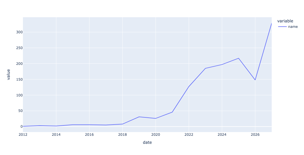
For reasons that aren't entirely clear to me, the x-axis labels are off by a tiny bit – so the line ends in 2026, and the label "2026" is actually where 2025 should be. But you don't need to read the x axis to see a huge spike over the last few years.
As you can see, the number of hacks, at least in this data set, has skyrocketed in the last year. And indeed, the number has risen pretty seriously (with the exception of last year) over the last few years. I'm going to guess that AI has something to do with this, but it's also possible that the large amount of money stored on crypto exchanges has something to do with it, too.
Create a line plot showing, for each year, the mean and median amounts of money (in USD) involved with each hack. Are the thieves getting more from each heist over time? Or are they just robbing more often?
Once again, I turned to resample. This time, I invoked it on the amount column, which reflects the value (in US dollars) of the heist when it took place. Because I wanted both the mean and median, I used agg and then passed those two aggregation methods as strings. And then, to reduce the number of digits after the decimal point, I invoked round:
(
    df
    .resample('1YE')['amount'].agg(['mean', 'median'])
    .round(2)
)
The result:
date	mean	median
2011-12-31	8750000.0	8750000.0
2012-12-31	189333.33	228000.0
2013-12-31	650000.0	650000.0
2014-12-31	81110000.0	3215000.0
2015-12-31	1654500.0	1189000.0
2016-12-31	27146000.0	2000000.0
2017-12-31	41264287.14	30000000.0
2018-12-31	44940479.68	500000.0
2019-12-31	13203739.48	7000000.0
2020-12-31	88388005.29	2000000.0
2021-12-31	23319103.84	3800000.0
2022-12-31	20645773.32	1225000.0
2023-12-31	8297211.07	714000.0
2024-12-31	8105326.29	708000.0
2025-12-31	18469534.82	840000.0
2026-12-31	28128016.4	490000.0
Now we can turn it into two line plots. I removed the call to round because there was no need for it here:
(
    df
    .resample('1YE')['amount'].agg(['mean', 'median'])
    .pipe(px.line)
)
The result:
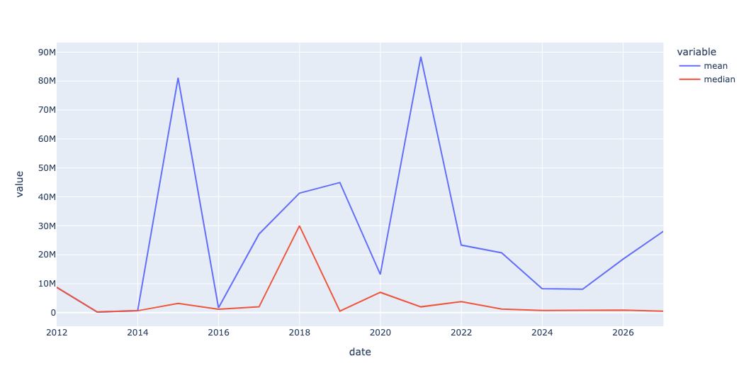
While the number of hacks has clearly gone up over time, but the amount stolen hasn't changed that much. What I find interesting is that with the exception of 2018, the median has stayed pretty constant – which means that the bulk are fairly low, with a few outliers. And indeed, the fact that the mean is often so much higher than the median demonstrates the power that the outliers have to pull it up.