


This week, in the wake of the US-Canada trade war (https://www.nytimes.com/2026/08/26/world/canada/carney-canada-trump-tariffs-retaliate.html?unlocked_article_code=1.8VA.peRW.DR9qdIs7xfTq&smid=url-share), I thought it might be interesting (and yes, a bit depressing) to read about the volume and type of trade that happens between the the two countries.
Data and five questions
This week's data comes from the Bureau of Transportation Statistics, whose transborder data is of particular use here:
https://www.bts.gov/topics/transborder-raw-data
They post a new zipfile every month – most recently from June 2026 – containing three CSV files describing the trade. We'll be looking at the second file (dot2) from each month, which lists what is being traded, the US state and Canadian province. We'll look at data from the 12 most recent downloadable files, from July 2025 through June 2026.
Paid subscribers, both to Bamboo Weekly and to my LernerPython+data membership program (https://LernerPython.com) get all of the questions and answers, as well as downloadable data files, downloadable versions of my notebooks, one-click access to my notebooks, and invitations to monthly office hours.
Learning goals for this week include working with multiple files, grouping, pivot tables, joins, and plotting with Plotly.
Here are my five questions and tasks for this week, along with my solutions and explanations:
Read all 12 files, from July 2025 through June 2026, into a Pandas data frame. Keep only the rows having to do with Canada. How much total value did the US export to and import from Canada? Draw a line plot showing total import and export for each month of last year.
Let's start by loading up what we'll need. In this case, it's not only Pandas and Plotly, but also pathlib from Python's standard library:
import pandas as pd
from plotly import express as px
from pathlib import Path
Why pathlib? Because I'll want to retrieve a number of different files from a multi-level directory tree matching a pattern. And yes, I could do that with the glob module from the standard library – but over the last few months, especially after Trey Hunner's talk at PyCon US, I've been trying to use pathlib instead of things like glob more and more — and I have to say, I'm enjoying it.
Next, I wanted to load the files. In theory, Pandas can retrieve a file via a URL, which means that I wouldn't need to download the 12 zipfiles to my computer, unzip them, and then retrieve the dot2 file from within each zipfile. But there's a catch there, namely that you can only use read_csv on a zipfile if it contains a single file. The moment several files are in the zipfile – which is a pretty common case, right? – then you cannot use that functionality.
So I downloaded all of the files into my usual data subdirectory under where my Bamboo Weekly notebooks live and unzipped them. I wanted to retrieve all of the dot2 files from within that tree; the idea was to invoke read_csv on each file, getting a list of data frames. I can then invoke pd.concat on the resulting list.
My strategy was thus to:
- Use
pathlibandglobto get a list of filenames - Iterate over each filename
- Run
pd.read_csvon each filename, resulting in a data frame - Use
pd.concatto combine all of these data frames together
All of this assumed, by the way, that it would be relatively easy to describe a globbing pattern that would handle all 12 files.
I started with a generator expression – a lazy form of list comprehension – to get all of the filenames (pathlib.Path objects, actually) matching my pattern. Notice that because pathlib is an object-oriented library, you cannot just invoke glob by itself; you need to invoke it on an existing Path object. And to do that, you need to give a filename or directory of some sort.
I thus created a Path object with the subdirectory in which this issue's data files were stored. Then, on that Path, I invoked glob, passing the pattern '/*dot2*.csv'. This returned each of the 12 files that I had downloaded into that subdirectory.
I then invoked read_csv on each of them; fortunately, they were all well behaved, and didn't need other options. However, given that I was going to read 12 files, and end up with over 1m rows, I decided to pass engine='pyarrow', in order to speed the loading and parsing:
(
    (pd.read_csv(one_filename, engine='pyarrow')
     for one_filename in Path('data/bw-185-bts-data/').glob('*/dot2*.csv'))
)
This worked fine, giving me a generator which gives me an iterable of data frames. I can thus pass this to pd.concat:
df = (
    pd.concat
    (pd.read_csv(one_filename, engine='pyarrow')
     for one_filename in Path('data/bw-185-bts-data/').glob('*/dot2*.csv'))
)
Sure enough, this gives me a data frame. But this data set contains information from both Canada and Mexico. And we're only interested in the data about Mexico. I can thus use dropna to remove rows that contain a NaN value in the CANPROV column, meaning those that don't have to do with Canada. Remember that dropna normally removes any row that has a NaN in it. By passing subset, we limit the rows that Pandas checks for NaN before removing it.
Remember that dropna also returns a new data frame, rather than modifying the existing one.
I also decided to drop two columns, MEXSTATE (since we won't have any Mexican states) and COUNTRY (since the only country we're dealing with here is Canada). I used drop, passing a list of column names to the columns keyword argument:
df = (
    pd.concat
    (pd.read_csv(one_filename, engine='pyarrow')
     for one_filename in Path('data/bw-185-bts-data/').glob('*/dot2*.csv'))
    .dropna(subset='CANPROV')
    .drop(columns=['MEXSTATE', 'COUNTRY'])
)
On my computer, this resulted in a data frame of 1,153,013 rows and 12 columns.
Next, I wanted to know how much total trade value there was between the US and Canada. Because this is a US data set, "import" means from Canada to the US, and "export" means from the US to Canada. That's in the TRDTYPE column, as described in the data dictionary on the BTS site, with a value of 1 for export (to Canada) and a value of 2 for import (from Canada).
This was a perfect case for groupby, using the sum aggregation method on the VALUE column. I then invoked apply, so that I could apply a string and the str.format method, to add a dollar sign, add commas between every group of three digits, and display 2 digits after the decimal point:
(
    df
    .groupby('TRDTYPE')['VALUE'].sum()
    .apply('${:,.02f}'.format)
)
The results:
TRDTYPE	VALUE
1	$994,420,917,017.00
2	$1,150,831,136,306.00
In other words:
- Over the last 12 months, the US has imported $994 billion in goods from Canada.
- Over the last 12 months, Canada has imported about $1.2 trillion in goods from the United States.
If this makes you wonder how that can be, with nearly even trade, it's important to remember that these are goods.
The US, as a general rule, imports a lot of goods, and exports far more services. Services, which many economists and commentators have pointed out, aren't addressed by Trump's tariffs.
Also, the fact that there is so much trade, going back and forth across the US-Canadian border, is because it's largely without any trade barriers.
Finally, I asked for a line plot for the total trade in each direction for each month of the last year. This required using groupby with two dimensions, both the MONTH column and the TRDTYPE column. I did that by grouping on a list of column names, rather than a single column name. Then, on the resulting multi-indexed series, I used unstack to move TRDTYPE to the columns.
I could have stopped there, invoking pipe and then px.line to get a nice line plot with two lines. But I was stuck with the legend of 1 and 2, which is far from intuitive. I thus used set_axis to rename the columns, indicating the direction of trade:
(
    df
    .groupby(['MONTH', 'TRDTYPE'])['VALUE'].sum()
    .unstack('TRDTYPE')
    .set_axis(['US->Canada', 'Canada->US'], axis='columns')
    .pipe(px.line)
)
The result:
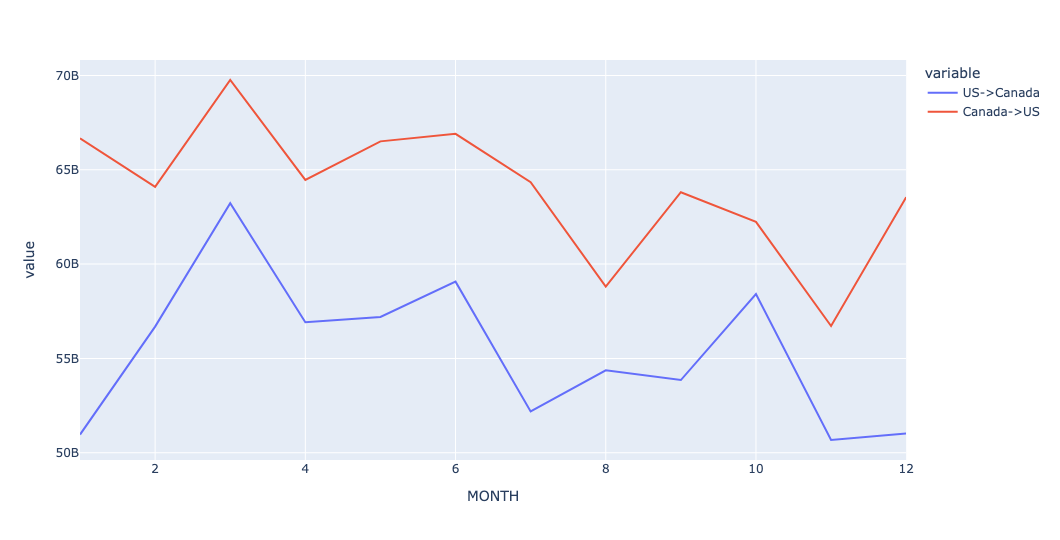
We can see that the US imports more from Canada than it exports to it, which seems to be part of why Trump believes the US is "losing" in trade with Canada. However, the numbers are fairly close together. This plot does also show a slow-and-small-but-steady drop in trade between the countries, but we would need many more years of data to know if this is because of the recent trade tensions or part of a larger trend.
Which 10 US states exported the most to Canada in the last year? Which imported the most? What are the biggest US state/Canadian province trading partners in each direction?
For starters, I used .loc and pd.col to keep only those rows where TDTYPE is 1, meaning export from the US to Canada. I then used groupby to get the sum of VALUE for each distinct state. Then I used nlargest to keep only the 10 states from which the exports were highest. Finally, I again used apply to get dollar signs and commas:
(
    df
    .loc[pd.col('TRDTYPE') == 1]
    .groupby('USASTATE')['VALUE'].sum()
    .nlargest(10)
    .apply('${:,.02f}'.format)
)
The result:
USASTATE	VALUE
DU	$139,833,001,333.00
TX	$106,415,431,428.00
MI	$65,447,148,487.00
IL	$53,284,944,504.00
OH	$52,021,378,540.00
NY	$49,892,090,635.00
CA	$49,710,463,948.00
PA	$40,805,512,112.00
IN	$38,140,290,842.00
KY	$25,334,902,891.00
The US state that exported the most to Canada is ... DU? I'm familiar with US state abbreviations, but this one stumped me a bit. Until I went to the data dictionary, and found that DU means "unknown." So from the perspective of BTS, $140b in exports to Canada can't be attributed to any given state.
I was surprised that Texas was the top-named state (after the Mystery State of DU), and we can use the data to examine just what they're exporting. But this is precisely what the Canadian government is hoping to exploit in this trade war: They know which US states voted for Trump and have endorsed his policies, and they will put heavy tariffs on goods coming from such states. It seems likely that Indiana, Kentucky, and Ohio, all of which export billions of dollars in goods to Canada, will find their produces are less welcome in Canada than they were before.
To get the reverse, we simply change the value for TRDTYPE from 1 to 2:
(
    df
    .loc[pd.col('TRDTYPE') == 2]
    .groupby('USASTATE')['VALUE'].sum()
    .nlargest(10)
    .apply('${:,.02f}'.format)
)
The results:
USASTATE	VALUE
IL	$174,440,974,425.00
MI	$130,347,695,012.00
TX	$101,649,563,176.00
NY	$61,611,239,066.00
OH	$49,633,641,364.00
WA	$48,290,499,484.00
CA	$47,226,027,398.00
PA	$40,294,074,581.00
MN	$38,593,958,222.00
IN	$31,221,222,705.00
We once again see many northern US states trading with Canada, as well as Texas and California. Many of these goods will be subject to the 50 percent tariff that Trump announced, and while not all are end-consumer goods, the effect will certainly be similar, namely raising prices on consumers in both countries.
Finally, I wanted to know which US state and Canadian province have the greatest total trade. To find out, I used pivot_table, putting the province abbreviations — not the standard ones, but BTS abbreviations — in the columns, the US state abbreviations in the index, and then add up the VALUE for each cell:
(
    df
    .pivot_table(columns='CANPROV',
                index='USASTATE',
                values='VALUE',
                aggfunc='sum')
)
That gave a nice table showing how much total trade there was between each state and province. To find the highest number, I first used agg with max and idxmax, to get the highest number and where it was. That resulted in a two-column data frame. I then used sort_values to find the highest number that was there:
(
    df
    .pivot_table(columns='CANPROV',
                index='USASTATE',
                values='VALUE',
                aggfunc='sum')
    .agg(['max', 'idxmax'], axis='columns')
    .sort_values('max', ascending=False)
)
The top 10 looked like this:
USASTATE	max	idxmax
MI	167001422185.0	XO
IL	136010372462.0	XA
DU	119389398797.0	OT
TX	102664688561.0	XO
NY	77011927539.0	XO
OH	69411471054.0	XO
IN	49686945860.0	XO
PA	49520840673.0	XO
CA	42446710888.0	XO
WA	29809919239.0	XC
In other words, the greatest trade was about $167b, between Michigan and the province of Ottawa. Second to that was Illinois, with about $136b in trade with Alberta.
To find out the greatest trading partners in each direction, we'll modify the above query using loc and pd.col to limit our interest to US-to-Canada trade:
(
    df
    .loc[pd.col('TRDTYPE') == 1]
    .pivot_table(columns='CANPROV',
                index='USASTATE',
                values='VALUE',
                aggfunc='sum')
    .agg(['max', 'idxmax'], axis='columns')
    .sort_values('max', ascending=False)
)
The winners:
USASTATE	max	idxmax
DU	110809069200.0	OT
MI	60349455721.0	XO
TX	46031154021.0	XO
OH	45195121854.0	XO
NY	40256920059.0	XO
IL	32527897678.0	XO
IN	31592184369.0	XO
PA	30524826367.0	XO
CA	27443574701.0	XO
KY	20923488227.0	XO
DU (unknown state) is doing a lot with OT, which is an unknown province. But in the #2 spot, we have Michigan and Ontario, followed by Texas and Ontario.
Or we can do Canada-to-US trade, which we get by flipping TRDTYPE from 1 to 2:
(
    df
    .loc[pd.col('TRDTYPE') == 2]
    .pivot_table(columns='CANPROV',
                index='USASTATE',
                values='VALUE',
                aggfunc='sum')
    .agg(['max', 'idxmax'], axis='columns')
    .sort_values('max', ascending=False)
)
Here are those results:
USASTATE	max	idxmax
IL	131998427529.0	XA
MI	106651966464.0	XO
TX	56633534540.0	XO
NY	36755007480.0	XO
MN	25189946375.0	XA
OH	24216349200.0	XO
WA	22118440603.0	XA
OK	20165884009.0	XA
PA	18996014306.0	XO
IN	18094761491.0	XO
In other words, people in Illinois buy from Alberta.