Bamboo Weekly #180: Movies (solutions)

This week, we took a break from the daily grind of current events to think about the movies. This was inspired by the flood of PR that I've seen and heard over the last week about the Odyssey, the new Christopher Nolan movie.

What's more, people are going to see the Odyssey in theaters, something that wasn't predicted during and after the covid-19 pandemic, which kept us all home and isolated, rather than in a crowded movie theater.

This got me wondering about how much the pandemic affected moviegoing, and how much theaters have bounced back since that time. And so, we'll examine data about movies, and particularly about movie theaters. Along the way, we'll look at which films and studios have done best, and what trends we're seeing.

Data and five questions

This week, we have data from two sources:

1. First, we have a data dump of movie revenues per day in the United States from January 1st, 2000 through January 3rd, 2025. This data, from Box Office Mojo, was collected and assembled at the GitHub repo https://github.com/tjwaterman99/boxofficemojo-scraper. Information about this large .csv.gz file (https://github.com/tjwaterman99/boxofficemojo-scraper/releases/latest/download/revenues_per_day.csv.gz) is on that page.
2. Second, we'll retrieve more recent daily data from Box Office Mojo using the boxoffice-api package (https://pypi.org/project/boxoffice-api/), whose get_daily method reads Box Office Mojo's daily chart. The package can optionally enrich each film with metadata (poster, plot, director, cast) from the OMDb API (https://www.omdbapi.com/) if you supply a free key — but that isn't needed for the revenue data here.

Paid subscribers, both to Bamboo Weekly and to my LernerPython+data membership program (https://LernerPython.com) get all of the questions and answers, as well as downloadable data files, downloadable versions of my notebooks, one-click access to my notebooks, and invitations to monthly office hours.

Learning goals for this week include working with APIs, combining data, dates and times, cleaning data, and grouping.

Here are my solutions and explanations for this week's questions:

Download the daily movie revenue file, and open it in a Pandas data frame. Ensure that the date column is a datetime and that it is the data frame's index. You can remove the id column. Based on this data, which movie earned the most total in each year in the data set? Create a bar plot from this data, showing the highest-grossing movie's revenue in each year. If you're using Plotly (and I believe you should!), put the movie's title in the tooltip.

I started off by loading up Pandas and Plotly, as well as the boxoffice-api package, which I downloaded and installed from PyPI:

import pandas as pd
from plotly import express as px
from boxoffice_api import BoxOffice 

I then used read_csv to open the file, and get a Pandas data frame back:

filename = 'data/bw-180-revenues.csv.gz'

df = (pd
    .read_csv(filename)
     )

You might be surprised that this worked. After all, .csv.gz means that it's not just a CSV file, but it's a compressed CSV file that was processed with GNU zip. That's a nice hidden feature in Pandas – that if it encounters a compressed file, it uncompresses it transparently, and then reads the data in the uncompressed version.

However, I wanted to do a few more things with this data frame: First, I wanted to remove the id column. I did that by invoking drop, passing the columns keyword argument and the column I wanted to remove:

filename = 'data/bw-180-revenues.csv.gz'

df = (pd
    .read_csv(filename)
    .drop(columns=['id'])
     )

Next, I wanted the date column to have a datetime dtype. Truth be told, I didn't think that this was necessary, because I originally used engine='pyarrow' to read the data into Pandas, and that gave me a column of type date. But it turns out that date columns don't support resample, which is needed to solve at least one problem in this list.

I thus used assign, giving a target column name of date. This means that we'll replace the existing date column with the new one. And the new one will be the result of invoking pd.to_datetime on the current contents of that column. Because the date is already in a standard format, we don't even have to specify the format; it just works.

Finally, I used set_index to make the date column our index, giving us what's often known as a "time series," where the index contains datetime values:

filename = 'data/bw-180-revenues.csv.gz'

df = (pd
    .read_csv(filename)
    .drop(columns=['id'])
    .assign(date = lambda df_: pd.to_datetime(df_['date']))
    .set_index('date')
     )

The result is a data frame with 356,322 rows and 4 columns.

I then asked to find which movie earned the most in each year of our data set. This seems like a straightforward and easy question, but it turns out to be surprisingly tricky to solve!

Let's start with the fact that we need to grab the year from the date column, but can't do that very easily, because it's currently being used as the index. I thus invoked reset_index to get it back as a regular column:

(
    df
    .reset_index()
)

I then, for the sake of convenience, used dt.year to grab the year from our date column, and used assign to create a new column that we can take advantage of:

(
    df
    .reset_index()
    .assign(year=pd.col('date').dt.year)
)

Next, I started on the grouping. I wanted to find out the total revenue for each movie in each year. Because year and title are separate columns, I ran groupby on both of them together, passing a list of column names (strings) rather than a single string.

Normally, groupby returns its results in a series or data frame with an index. Here, we don't want that, so I used as_index=False:

(
    df
    .reset_index()
    .assign(year=pd.col('date').dt.year)
    .groupby(['year', 'title'], as_index=False)['revenue'].sum()
)

This returns a 3-column data frame (year, title, and revenue) reflecting the amount that each movie made in each year. We only want the highest-revenue movie from each year, though. To get that, I first used sort_values to sort the data frame in order of revenue, from smallest to largest. I then invoked drop_duplicates, which returned our data frame but without any duplicated years.

But wait – if it does have multiple rows with the same year, what should it do? Which should it keep? I passed keep='last', which means that the final row with each year should be kept – which, thanks to our sort_values invocation from before, is guaranteed to be the highest-revenue movie from each year:

(
    df
    .reset_index()
    .assign(year=pd.col('date').dt.year)
    .groupby(['year', 'title'], as_index=False)['revenue'].sum()
    .sort_values('revenue')
    .drop_duplicates('year', keep='last')
)

I finished this up by invoking sort_values again, to sort by year. And then I got rid of the irrelevant integers in our index with reset_index, adding drop=True so that the index isn't put into our data frame:

(
    df
    .reset_index()
    .assign(year=pd.col('date').dt.year)
    .groupby(['year', 'title'], as_index=False)['revenue'].sum()
    .sort_values('revenue')
    .drop_duplicates('year', keep='last')
    .sort_values('year')
    .reset_index(drop=True)
)

So, what movie earned the most in each year of our data set? In trying to display it outside of Marimo, I realized that I would like to add a $ before the number and commas between the digits. I thus added a call to apply from within the assign call:

(
    df
    .reset_index()
    .assign(year=pd.col('date').dt.year)
    .groupby(['year', 'title'], as_index=False)['revenue'].sum()
    .sort_values('revenue')
    .drop_duplicates('year', keep='last')
    .sort_values('year')
    .reset_index(drop=True)
    .assign(revenue = pd.col('revenue').apply('${:,}'.format))
)

The results:

year	title	revenue
2000	How the Grinch Stole Christmas	$251,628,905
2001	Harry Potter and the Sorcerer's Stone	$288,641,892
2002	Spider-Man	$401,487,933
2003	Finding Nemo	$335,298,792
2004	Shrek 2	$436,721,703
2005	Star Wars: Episode III - Revenge of the Sith	$380,270,577
2006	Pirates of the Caribbean: Dead Man's Chest	$419,867,749
2007	Spider-Man 3	$336,104,636
2008	The Dark Knight	$530,924,926
2009	Transformers: Revenge of the Fallen	$402,111,870
2010	Avatar	$466,141,929
2011	Harry Potter and the Deathly Hallows: Part 2	$381,011,219
2012	The Avengers	$619,257,177
2013	Iron Man 3	$406,609,688
2014	Guardians of the Galaxy	$328,095,589
2015	Jurassic World	$652,197,981
2016	Finding Dory	$486,295,561
2017	Star Wars: Episode VIII - The Last Jedi	$517,218,368
2018	Black Panther	$700,059,566
2019	Avengers: Endgame	$858,373,000
2020	Bad Boys for Life	$204,417,855
2021	Spider-Man: No Way Home	$572,507,143
2022	Top Gun: Maverick	$716,981,130
2023	Barbie	$636,829,566
2024	Inside Out 2	$650,924,793
2025	Mufasa: The Lion King	$24,220,986

Data for 2025 is much smaller than other years, because the data only goes through January. But it seems pretty obvious, from these titles and numbers, why so many studios are making superhero movies.

To create a bar plot from this data, I replaced the final assign line above with a new one, using pipe to invoke px.bar as part of the method chain. I passed three keyword arguments to pipe, which were then passed along to px.bar: x, indicating which column should contain the x axis, y, indicating which column should be used for the y axis, and hover_data, indicating which column(s) should be displayed when the user hovers over the bar:

(
    df
    .reset_index()
    .assign(year=pd.col('date').dt.year)
    .groupby(['year', 'title'], as_index=False)['revenue'].sum()
    .sort_values('revenue')
    .drop_duplicates('year', keep='last')
    .sort_values('year')
    .reset_index(drop=True)
    .pipe(px.bar, x='year', y='revenue', hover_data='title')
)

The result:

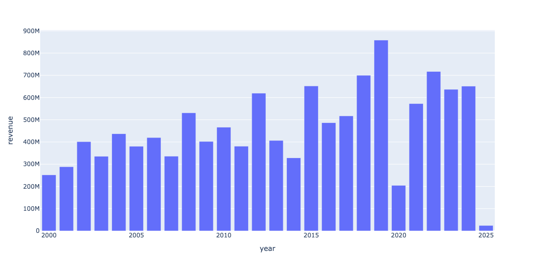
As you can see, the top-grossing movies were (overall) doing better and better over the years... until we got to 2020, the first full year of the covid-19 pandemic, and the revenues were obviously quite low.

Create a line plot showing, for each year in the data set, the total revenue from all movies in the data set. Do you see the effect of the pandemic? According to this data, have we surpassed pre-pandemic movie revenue yet? (You can ask this again in question 5, if you want, after adding some more data.)

What if we are interested in all of the movie revenue for each year? That turns out to be much simpler than what we just did. In theory, we could use a groupby. But I often prefer to use resample, which is a bit different and more flexible – basically, resample requires that our index contain datetime values.

We can then ask to break time up into any level of granularity we want. So if I want annual data, I can give it the specifier '1YE', for "1 year end." You can use any number you want, and use a variety of different time measurements, such as months, weeks, and minutes. The combination can be quite powerful.

Here, I first invoked resample, asking to sum the revenue column on an annual basis. I then passed the resulting data frame directly to pipe, which passes it along to the px.line method:

(
    df
    .resample('1YE')['revenue'].sum()
    .pipe(px.line)
)

Here's the result:

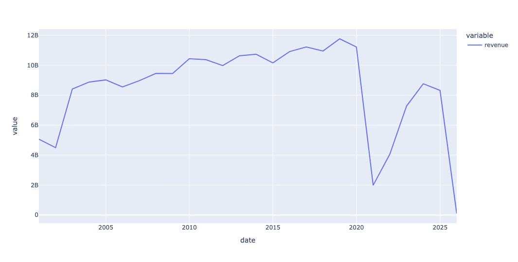
This is the total revenue number reported per year, And you can see the extreme dip that happened in 2020 and 2021 as people either didn't want to go to the movies or weren't allowed to do so.

We can also see that 2024 certainly continues the positive trend among moviegoers, but we still aren't back to where we were in the pre-pandemic era.