


Yesterday, I wrote that the Federal Reserve was almost certainly going to lower interest rates, and that there was discussion over whether they would lower them by a quarter point or half a point. In the end, the Fed lowered rates by half a point (https://www.nytimes.com/2024/09/18/business/economy/fed-reserve-interest-rate-cut.html?unlocked_article_code=1.L04.bMvn.prjPbTGVNwJZ&smid=url-share), and signaled that they will likely cut rates even more over the coming year. This doesn't mean that the economy is doing poorly, merely that they were able to slow it down and reduce inflation without pushing the US into a recession – a so-called "soft landing."
This week, we looked at data from the Bank of Bank of International Settlements (BIS, http://bis.org/), a sort of central bank for central banks. They collect data from central banks around the world, making it easy for us to compare interest rates, as well as who changed them, by how much, and when.
Data and six questions
BIS makes it fairly easy to retrieve the data we want in CSV format. You can go to their data site, at
https://data.bis.org/topics/CBPOL/data
and click on "export." You can choose to download the data in CSV from
https://data.bis.org/static/bulk/WS_CBPOL_csv_col.zip
Or you can click on "code snippet," getting Pandas code that will allow you to download the data, via the BIS API, into Pandas. I found that downloading multiple times in a row will result in your computer not being able to download any more; they seem to have some sort of limiting system.
[Note: I got something wrong with the above URLs and instructions. I'm not quite sure what, but I've put the file that I intended for you to download at https://files.lerner.co.il/central-bank-data.csv.zip .My apologies!]
I gave you six tasks and questions this week. A link to the Jupyter notebook I used to solve the problems is at the bottom of this post. Here, meanwhile, are my solutions and explanations:
Create a data frame from the BIS data. Keep only the rows in which TIME_PERIOD has two - characters. Turn the remaining values in TIME_PERIOD into datetime values, and then keep only those rows starting in the year 2000.
Let's start by loading Pandas:
import pandas as pdNext, I'll admit that I cheated a bit – after finding that they blocked my computer from downloading the BIS file after a few times, I just downloaded it onto my machine, stuck it into my "downloads" directory, and was done with it. But I assure you, it is possible to download the zipfile and open it!
Indeed, it's always useful to remember that if you pass a CSV file with a .csv suffix to read_csv, everything will work fine. But if you pass a file with a .csv.zip suffix to read_csv, Pandas will unzip the zipfile and extract the CSV that it contains.
So let's start by setting a url variable (which will just contain a filename), and using read_csv to get a data frame from it:
url = '/Users/reuven/Downloads/central-bank-data.csv.zip'

df = (
    pd
    .read_csv(url)
)
This sort of works, but at least on my computer, I got a warning. If we don't specify the dtype of columns in the input file, then Pandas has to look at a large number of rows to determine (well, guess) the dtype that it'll give to each column. It does this in chunks, and if an earlier chunk disagrees with a later chunk, you'll get that warning.
But the warning also suggests two solutions: One is to pass the dtype keyword argument, specifying a dtype for each column. The other is to pass low_memory=False as a keyword argument. This tells Pandas that we have enough memory on our computer to load the whole thing at once, thus allowing its guess to be more accurate. That's what I decided to do:
df = (
    pd
    .read_csv(url, low_memory=False)
)
The good news is that we now have a data frame with all of the data from the input CSV file. However, I asked you to keep only those date columns with two "-" characters. (I could have said that each date needed to have a year, month, and day, but decided to be kind, with a specific instruction.) We need to do this so that all of the elements in the TIME_PERIOD column will be in a format that can be turned into a datetime value.
How, then, can we keep only rows in which the TIME_PERIOD has two "-" characters? We can use str.count on a string data frame, telling us how many times a character appears in a string. We can then compare that output with 2., getting a boolean series back. And we can wrap that condition inside of a combination of loc and lambda:
df = (
    pd
    .read_csv(url, low_memory=False)
    .loc[lambda df_: df_['TIME_PERIOD'].str.count('-') == 2]
)
When the above query is done, we have a data frame with a TIME_PERIOD column that is still a string, but at least it can be turned into datetime values.
But now we have another problem: To take a series of strings and get back a series of datetime values, we need to call pd.to_datetime. There's nothing wrong with that, per se – but we're doing method chaining, and to_datetime is a function. We could break the chain, assigning the result of the loc to a variable, and then invoking pd.to_datetime on that variable.
But we can do something else, instead: We can use assign, a method that lets us (temporarily) create a new column on a data frame. If the column has the same name as an existing column, then the old one is replaced with the new one. We do this by calling assign with a keyword argument. The keyword name is the name of the column we want to create (or update), and the value is whatever value we want to provide. Or it can be a lambda expression, in which case the result of the lambda is the new column value.
I used this to transform the TIME_PERIOD column into a datetime value:
df = (
    pd
    .read_csv(url, low_memory=False)
    .loc[lambda df_: df_['TIME_PERIOD'].str.count('-') == 2]
    .assign(TIME_PERIOD = lambda df_: pd.to_datetime(df_['TIME_PERIOD']))
)
We now have a data frame in which TIME_PERIOD is a datetime, and the other columns are (we'll assume) the values and types that we want. However, I did ask you to do one more thing, namely to keep only those rows from the year 2000 and onward.
We can do that with yet another loc - lambda combination, this time using the dt accessor to retrieve a component of the date and time – the year, using dt.year. Wherever the year is greater than or equal to 2000, we'll keep the row:
url = '/Users/reuven/Downloads/central-bank-data.csv.zip'

df = (
    pd
    .read_csv(url, low_memory=False)
    .loc[lambda df_: df_['TIME_PERIOD'].str.count('-') == 2]
    .assign(TIME_PERIOD = lambda df_: pd.to_datetime(df_['TIME_PERIOD']))
    .loc[lambda df_: df_['TIME_PERIOD'].dt.year >= 2000]
)
The result is a data frame with 316,437 rows and 15 columns.
What is the latest interest rate for each central bank? Which five banks have the highest interest rates in the world, and which have the lowest?
Next, I asked you to find the most recent interest rate for each central bank. Originally, I thought that this would be pretty straightforward. After all, we presumably get updates from each bank on a regular schedule, We just take the interest rate from each bank on the most recent date in the database, and it'll be great! (Spoiler alert: No, it won't.)
I decided that to rejigger our data into a new data frame, one in which the rows contain dates and the columns contain the names of central banks. Then, the thinking went, we could retrieve the final row from the data frame, and get the most recent value for each central bank.
How can I rewrite the data frame in this way? It's actually a pivot table! We can invoke pivot_table as follows:
- The rows will be the dates from the
TIME_PERIODcolumn - The columns will be the central bank names from the
SOURCE_REFcolumn - The values will be the
OBS_VALUEfor each intersection of bank and date
Then we can grab the final row, and we'll know the current rate for each central bank:
(
    df
    .pivot_table(index='TIME_PERIOD', columns='SOURCE_REF', values='OBS_VALUE')
    .iloc[-1]
)
The good news? We get a series with central bank names as the index, and interest rates as the values.
The bad news? We end up with a bunch of NaN values, because not every central bank reports rates on the same schedule. Only those banks that reported on the final day in the data set (September 10th, 2024 in the version I retrieved) will have a value.
Missing data is always an issue in data analysis, and this is a good example of having to work with it. The thing is, we know that if a central bank announces a new interest rate on September 1st, and doesn't announce any new rates after, we should use the September 1st rate for all subsequent days. In other words, we want to fill the NaN values with whatever the previous non-NaN value was.
Pandas provides a ffill method ("forward fill") that performs precisely this type of action. If we run it on a data frame, then any NaN will be replaced by the most recent non-NaN value. This will be true for the entire data frame, even though we're only interested in the final NaN values. We can thus say:
(
    df
    .pivot_table(index='TIME_PERIOD', columns='SOURCE_REF', values='OBS_VALUE')
    .ffill()
    .iloc[-1]
)
We get the final row with iloc, asking for index -1, meaning the final one. The rates, in the data set that I got, were:
SOURCE_REF
Bangko Sentral ng Pilipinas                    6.250
Bank Al-Maghrib (Central Bank of Morocco)      2.750
Bank Indonesia                                 6.250
Bank Negara Malaysia                           3.000
Bank of Canada                                 4.250
Bank of England                                5.000
Bank of Israel                                 4.500
Bank of Japan                                  0.250
Bank of Korea                                  3.500
Bank of Mexico                                10.750
Bank of Russia                                18.000
Bank of Thailand                               2.500
Central Bank of Argentina                     40.000
Central Bank of Brazil                        10.500
Central Bank of Chile                          5.500
Central Bank of Colombia                      10.750
Central Bank of Iceland                        9.250
Central Bank of the Republic of Turkey        50.000
Central Reserve Bank of Peru                   5.500
Croatian National Bank                         0.000
Czech National Bank                            4.500
Danmarks Nationalbank                          3.350
European Central Bank                          4.250
Hong Kong Monetary Authority                   5.750
Hungarian National Bank                        6.750
National Bank of Poland                        5.750
National Bank of Romania                       6.500
National Bank of Serbia                        6.000
National Bank of the Republic of Macedonia     6.300
Norges Bank                                    4.500
People's Bank of China                         3.350
Reserve Bank of Australia                      4.350
Reserve Bank of India                          6.500
Reserve Bank of New Zealand                    5.250
Saudi Arabian Monetary Authority               6.000
South African Reserve Bank                     8.250
Sveriges Riksbank                              3.500
Swiss National Bank                            1.250
US Federal Reserve System                      5.375
Name: 2024-09-10 00:00:00, dtype: float64
Notice that the central bank names are alphabetized. That's because pivot_table , by default, sorts its output by the index.
Now that we have this information, we can ask which are the five banks with the highest rates in the world, and which have the lowest rates in the world. We could invoke nsmallest and nlargest on the above series, but why not do them both at once, thanks to agg?
(
    df
    .pivot_table(index='TIME_PERIOD', columns='SOURCE_REF', values='OBS_VALUE')
    .ffill()
    .iloc[-1]
    .agg(['nlargest', 'nsmallest'])
)
I got the following output:
                                           nlargest  nsmallest
SOURCE_REF
Central Bank of the Republic of Turkey        50.00        NaN
Central Bank of Argentina                     40.00        NaN
Bank of Russia                                18.00        NaN
Bank of Mexico                                10.75        NaN
Central Bank of Colombia                      10.75        NaN
Croatian National Bank                          NaN       0.00
Bank of Japan                                   NaN       0.25
Swiss National Bank                             NaN       1.25
Bank of Thailand                                NaN       2.50
Bank Al-Maghrib (Central Bank of Morocco)       NaN       2.75
We can see that Turkey and Argentina (not surprisingly) have the highest interest rates, followed by Russia, Mexico, and Colombia. The lowest interest rates are in Croatia and Japan, followed by Switzerland, Thailand, and Morocco.
Notice that when we use agg, we get one column for each of the aggregation methods we invoked. In the case of nsmallest and nlargest, it's rare for the two to overlap – so we get NaN values in one column when the other has values.
Create a table in which each row represents the last day in each month, each column represents a central bank, and each data cell represents the highest rate during that month.
To solve this, we can use the resample method on the pivot table we created in the previous solution, after the subsequent call to ffill. Resampling only works when the data frame's index is a datetime value – but the pivot table is just like that, so we're fine.
Resampling is a kind of time-based groupby operation. We indicate the time granularity by which we want to group the results, the column(s) on which we want to perform a calculation, and the aggregation method(s) we want to run. Here, we want to get the highest value (i.e., max) of the rates (i.e., OBS_VALUE), at the end of each month (i.e., the resampling code 1ME, for "end of one month"):
(
    df
    .pivot_table(index='TIME_PERIOD', columns='SOURCE_REF', values='OBS_VALUE')
    .ffill()
    .resample('1ME').max()
)
The result is a data frame whose index contains the final day of each month (thanks to the 1ME format code), and whose values are the highest during that period.
Use the data from question 3 to plot reserve-bank rates for the US, Canada, European Central Bank, India, China, and Japan. Which central bank has consistently had the lowest rates? Which has had the highest? What major rises and falls across banks do we see?
If we start with the output from resample in the previous question, we know that the central banks' names are in the columns. We can thus use [] to retrieve a list of columns that interest us, from the banks I mentioned:
(
    df
    .pivot_table(index='TIME_PERIOD', columns='SOURCE_REF', values='OBS_VALUE')
    .ffill()
    .resample('1ME').max()
    [['Bank of England', 'US Federal Reserve System', 'European Central Bank',
     'Reserve Bank of India', 'Bank of Canada', 'Bank of Japan']]
)
We can then plot all six of these banks' rates over time by invoking plot.line on our data frame:
(
    df
    .pivot_table(index='TIME_PERIOD', columns='SOURCE_REF', values='OBS_VALUE')
    .ffill()
    .resample('1ME').max()
    [['Bank of England', 'US Federal Reserve System', 'European Central Bank',
     'Reserve Bank of India', 'Bank of Canada', 'Bank of Japan']]
    .plot.line()
)
We get the following plot:
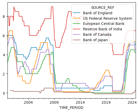
We can see that the Reserve Bank of India has kept interest rates high for a long time, and that the Bank of Japan has kept them quite low for a long time, as well. Other than those two – and even, to some degree, in the case of India – we see a major fall at the start of 2009, when the major financial crisis hit the United States, and then the world. And we also see a sharp drop at the start of 2020, when the covid-19 pandemic started, followed by a rise in most of the banks as the pandemic receded and inflation kicked in for the first time in a generation.
Calculate the month-over-month change in interest rates for each central bank. Were there any months in which a majority of banks all lowered their rates from the previous month?
To find out whether a majority of banks lowered rates from the previous month, we'll start with the monthly rates that we got from invoking resample in the previous solution. We'll then run pct_change, to get the percentage change that each cell had from the one above it. The resulting data frame will tell us, for each month and central bank, the degree to which the rates changed.
(
    df
    .pivot_table(index='TIME_PERIOD', columns='SOURCE_REF', values='OBS_VALUE')
    .ffill()
    .resample('1ME').max()
    .pct_change()
)
But we don't really care about the percentage change. Rather, we care about whether the change was negative, i.e., the banks lowered their rates. To do that, we'll want to find out which cells contain a negative value. Normally, we would do that with the < operator. But here, we'll use the method equivalent, lt .
The result is a data frame equivalent to our resampling result, but with True and False values to indicate if the rate was lower (True) or higher (False) than the previous month:
(
    df
    .pivot_table(index='TIME_PERIOD', columns='SOURCE_REF', values='OBS_VALUE')
    .ffill()
    .resample('1ME').max()
    .pct_change()
    .lt(0)
)
Now comes the trickiest part: We're going to use loc and lambda again, to retrieve only selected rows from our boolean data frame. Which rows? Those in which the sum of values in the row is more than 20.
When we invoke sum on a data frame of boolean values, the True values are treated as 1, and the False values are treated as 0. The result of invoking sum will normally thus give us the number of True values in a column. However, we want to calculate this by the rows, so we pass the axis='columns' keyword argument to sum:
(
    df
    .pivot_table(index='TIME_PERIOD', columns='SOURCE_REF', values='OBS_VALUE')
    .ffill()
    .resample('1ME').max()
    .pct_change()
    .lt(0)
    .loc[lambda df_: df_.sum(axis='columns') > 20]
)
I then invoked index on this, to get the current index values. The result:
DatetimeIndex(['2009-01-31', '2009-04-30', '2020-04-30'], dtype='datetime64[ns]', name='TIME_PERIOD', freq=None)We can see that on January 31st, 2009, April 30th, 2009, and April 30th, 2020, a majority of central banks around the world all reduced their rates. And as mentioned earlier 2009 was the financial crisis and 2020 was the pandemic, both good reasons for the Fed to try to stabilize things.
The US Federal Reserve is considered the most influential central bank in the world. When it raises or lowers rates, other banks consider doing so, too. Calculate the correlation between the rise or drop in Fed rates and those in other central banks, delayed by 2 months. Which five banks move most consistently with the Fed, but with a two-month delay?
Finally, this seemed like an interesting real-world question, as well as a challenge to solve with Pandas. First, I'll define a variable, lag_factor, indicating by how many months I want to look for a delayed correlation:
lag_factor = 2Now we can use this variable, and experiment with different lags.
We'll again go through creating our pivot table, filling, resampling, and getting the percentage change with each month.
I'll then want to run corr, to find the correlations between the Fed's rates and other rates. But actually, I want to run corr on the shifted rates. One way to do this is to replace the existing Fed column with a new one with shifted values.
I'll use assign for this, but because the Fed column contains spaces, its name isn't a legal Python identifier. I'll thus create a new column, named lagged_fed, and use shift to put NaN values in the first two rows (thanks to lag_factor) of that column. I then use drop to remove the old column, which we don't need any more:
(
    df
    .pivot_table(index='TIME_PERIOD',
                 columns='SOURCE_REF',
                 values='OBS_VALUE')
    .ffill()
    .resample('1ME').max()
    .pct_change()
    .assign(lagged_fed=lambda df_:
            df_['US Federal Reserve System'].shift(lag_factor))
    .drop('US Federal Reserve System', axis='columns')
)
After running corr, we have a full data frame with the correlations. All we want are the correlations with the Fed, so we'll retrieve just the lagged_fed column. That gives us a series on which we can run nlargest, to get the five largest correlations:
(
    df
    .pivot_table(index='TIME_PERIOD',
                 columns='SOURCE_REF',
                 values='OBS_VALUE')
    .ffill()
    .resample('1ME').max()
    .pct_change()
    .assign(lagged_fed=lambda df_:
            df_['US Federal Reserve System'].shift(lag_factor))
    .drop('US Federal Reserve System', axis='columns')
    .corr()
    ['lagged_fed']
    .nlargest()
)
The result that I got was:
SOURCE_REF
lagged_fed                          1.000000
Reserve Bank of Australia           0.544483
Hong Kong Monetary Authority        0.421295
Saudi Arabian Monetary Authority    0.366124
Sveriges Riksbank                   0.360133
Name: lagged_fed, dtype: float64
We see that there is a positive delayed correlation between the Fed's actions and central banks in those in other countries. It's not overwhelming, but it does exist.
My Jupyter notebook for this week is here: https://drive.google.com/file/d/1CSpoIcIV-bDsSqKkXwC3QPOZZzrzKGEi/view?usp=sharing
I'll be back on Wednesday of next week with more Pandas puzzles based on current events.
Reuven