


This week, we celebrated (mourned?) the start of the school year in much of the northern hemisphere, looking at trends in education for various countries and regions in the world. There's no end to the questions that we can ask about education, ranging from the financial investment to the number of students who start school to the number of graduates to the quality of teaching. The good news is that governments and international organizations collect a large amount of data about schools and education, allowing us to look into what techniques and systems do (and don't) work.
I found an interesting dataset from the World Bank (https://worldbank.org), which helps low-income countries to invest in infrastructure and education. However, its data reflects the entire world, not just the countries where it invests, allowing us to identify trends and make comparisons.
Data and six questions
And indeed, we start this week's data journey at the World Bank's educational data page:
https://data.worldbank.org/topic/education
You can explore their educational data in your browser, but we're here to retrieve and work directly with it using Pandas. To retrieve the data, you can click on the "CSV" link on that page, or just download it directly from
https://api.worldbank.org/v2/en/topic/4?downloadformat=csv
The download contains three CSV files, not one. The first (and main) one contains the data itself, while the two other CSV files contain metadata about the indicators and metadata about the countries. You'll need all three to answer this week's questions.
I gave you six questions and tasks for this week. Here are my solutions; a link to the Jupyter notebook that I used is at the bottom of this post:
Import the main file into a data frame. Set its index to be the "Country Code" column, drop the "Unnamed: 68" column, and keep only those rows where "Indicator Code" starts with "SE.".
Before we do anything else, let's load up Pandas:
import pandas as pdIn theory, we can just use read_csv to read a CSV file into a data frame:
main_filename = 'API_4_DS2_en_csv_v2_3434744.csv'

df = (pd
      .read_csv(main_filename)
     )
However, if we try to do it this way, we'll get an error message. That's because the before the data starts, the file contains some comments. The CSV parser assumes that those comments are data, infers (incorrectly) how many columns the file contains, and then gives us an error message when it encounters the actual data.
The solution is to tell read_csv that it should skip several lines, and that the headers for the data actually start on the third line of the file – which we describe as "line 2" when we start counting with 0:
main_filename = 'API_4_DS2_en_csv_v2_3434744.csv'

df = (pd
      .read_csv(main_filename, header=2)
     )
This is fine, except that we now have the entire data set, when we're really interested in looking at education-specific indicators. Those indicators' codes all start with the string "SE.", so I asked you to keep only lines with such indicators.
We can do that by using the str accessor to execute a string method (str.startswith) on each of the rows, getting back a boolean values (True or False) for each indicator code. Feeding that boolean value back into a combination of loc and lambda returns only the matching rows:
main_filename = 'API_4_DS2_en_csv_v2_3434744.csv'

df = (pd
      .read_csv(main_filename, header=2)
      .loc[lambda df_: df_['Indicator Code'].str.startswith('SE.')]
     )
People often ask why I use df_ as the variable in my lambda expression, rather than the more standard df. I always say that there are two reasons: First, so that we don't get confused between the global variable df and the local variable (i.e., parameter) df_, which only exists in the context of the running function.
The second reason is that when we chain our methods in this way, each method is running on the result of the previous one. We're purposely not assigning each intermediate step to a variable; the whole point is that we'll run a number of methods, each modifying the data frame in some way, until the final method is run, when we'll assign or view the final result. So even if we would want to refer to the global data frame from within the lambda, there isn't any variable to refer to.
That's even truer in this case, where df isn't defined until the final method runs. We're running .loc on the result of read_csv, before any variable has been defined or is available.
The result is a data frame with 39,634 rows and 69 columns. Why so many? Each row represents a single measure for a single country or region. Aside from the columns indicating which country/region and indicator we're talking about, we have columns for each year during which the World Bank collected data, starting in 1960. There isn't data for every country/region for each year; we'll remove some of that missing data in just a bit.
Import the two metadata files into data frames, and join them together with the main data frame. Remove any columns that start with the word "Unnamed". Then make the country code into the index.
The data itself is interesting, but the two metadata files allow us to dig even deeper. We'll thus join the three CSV files together into a single, large data frame. (Note that we'll only really use one of the files to answer our questions; part of the reason for me posing this question was to give you more practice with joins.)
Pandas has two methods that we can use to join data frames together:
join, which uses the index to combine them, much as we would in SQL, andmerge, which lets join data frames using any columns we want, not just the index.
The difference between the two isn't that great, given that we can use any column in a data frame as its index.
First, I decided to combine df with the country metadata. I loaded the country metadata into a data frame:
country_filename = 'Metadata_Country_API_4_DS2_en_csv_v2_3434744.csv'

(
    pd
    .read_csv(country_filename)
)
But I don't really need this data frame on its own; the only reason I'm reading it into Pandas at all is to combine it with df. Both df and the country metadata have a Country Code column, so I can invoke merge on that, assigning the resulting data frame to df:
country_filename = 'Metadata_Country_API_4_DS2_en_csv_v2_3434744.csv'

df = (
    pd
    .read_csv(country_filename)
    .merge(df, on='Country Code')
)
df now contains all of the columns from both the full data set and the country-related metadata. However, we see that the new df has 149 fewer rows than we had in the original df. This is because the default behavior is to perform an "inner join," only producing a result row where both input data frames match up. If a country code exists in one data frame, but not the other, then there is no match, and no resulting row.
If we had used an "outer join," then we would have the same number of rows as in the input, with NaN values wherever there wasn't a match.
By the way, what country appeared in one but not the other? I used Python's set class to find out:
set(
    pd
    .read_csv(country_filename)
    ['Country Code']
) ^ set(df['Country Code'])
It returned a single item, INX, which appears in the main data file. The country name associated with INX is... "Not classified." I'm just fine leaving it out of my final data frame, and sticking with the inner join.
However, we're not quite done: We also need to merge in the indicators metadata. However, we can't specify the name of the column that's common to both df and the indicator CSV file, because they use slightly different names: df uses Indicator Code, and the indicator metadata file uses INDICATOR_CODE. Fortunately, we can tell merge the names of the columns we want to use with the left_on and right_on keyword arguments:
indicator_filename = 'Metadata_Indicator_API_4_DS2_en_csv_v2_3434744.csv'

df = (
    pd
    .read_csv(indicator_filename)
    .merge(df, left_on='INDICATOR_CODE', right_on='Indicator Code')
)
If it's not obvious which one is "left" and which one is "right" here, remember that we're invoking the merge method on the indicator metadata's data frame, which makes it the "left" data frame. The right data frame is df, the data frame we created before.
The final data frame still has 39,485 rows, which means that matches were found for all of the indicator codes.
Could we do all of this in a single, chained method call? Yes!
df = (pd
      .read_csv(main_filename, header=2)
      .loc[lambda df_: df_['Indicator Code'].str.startswith('SE.')]
      .merge(pd.read_csv(country_filename),
             on='Country Code')
      .merge(pd.read_csv(indicator_filename),
             left_on='Indicator Code', right_on='INDICATOR_CODE')
     )
The biggest change here is that I'm calling merge on the original df (rather than on the country data frame), and then on the result of that merge (rather than on the indicator data frame). This means that the notions of "left" and "right" are swapped, so I have to switch the values in left_on and right_on. But other than that, this works just fine, and we get the same result.
Finally, I asked you to remove all of the column that start with "Unnamed." We can do that by invoking df.drop, passing a list of columns we want to remove (and specifying axis='columns').
Finally, I then used set_index to set the index of the data frame to the country code:
df = (pd
      .read_csv(main_filename, header=2)
      .loc[lambda df_: df_['Indicator Code'].str.startswith('SE.')]
      .merge(pd.read_csv(country_filename),
             on='Country Code')
      .merge(pd.read_csv(indicator_filename),
             left_on='Indicator Code', right_on='INDICATOR_CODE')
      .drop(['Unnamed: 68', 'Unnamed: 5', 'Unnamed: 4'],
            axis='columns')
      .set_index('Country Code')
     )
What 10 countries had, in 2022, the highest percentage of female bachelor's degree or better?
With our data frame now in place, we can start to ask some questions regarding the educational content. For example, one measure of a country's development is the percentage of educated girls and women. So my first question is which countries, in 2022, had the highest percentage of women with a bachelor's degree.
In order to answer this, we first need to find that indicator. Searching through the various indicator names and codes, I found it was SE.TER.CUAT.BA.FE.ZS. (Who comes up with these codes, anyway?)
First, then, we'll keep only those rows with that indicator code. Moreover, we'll only need the data from 2022 and the name of the country (to make it easier to read the results). We can thus use the two-argument form of .loc, the first being a row selector (here, again, using lambda) and the second being the column selector (here, being a list of two column names):
(
    df
    .loc[lambda df_: df_['INDICATOR_CODE'] == 'SE.TER.CUAT.BA.FE.ZS',
        ['2022', 'Country Name']]
)
Next, we can set the index to be Country Name – again, not for any technical reason, but just to make the results a bit easier to read and understand:
(
    df
    .loc[lambda df_: df_['INDICATOR_CODE'] == 'SE.TER.CUAT.BA.FE.ZS',
        ['2022', 'Country Name']]
    .set_index('Country Name')
)
Next, I used dropna to remove any empty values from the one remaining column in our data frame. Note that the column name is not the integer 2022, but rather the string '2022', so we need to use the quotes whenever we refer to it.
Next, we can then sort the values in descending order, using head to retrieve the top 10:
(
    df
    .loc[lambda df_: df_['INDICATOR_CODE'] == 'SE.TER.CUAT.BA.FE.ZS',
        ['2022', 'Country Name']]
    .set_index('Country Name')
    .dropna()
    .sort_values('2022', ascending=False)
    .head(10)
)
Here's what I got for results:
                           2022
Country Name
United Arab Emirates  51.812222
Qatar                 49.104580
Lithuania             46.154793
Iceland               41.947754
Israel                41.732250
Belgium               41.254791
Luxembourg            41.212471
Australia             40.023781
United States         39.008301
Sweden                38.991272
In 2022, what countries had the highest literacy rate for adult males and females? The lowest?
Next, I was curious to know what the literacy rates were for males and females – and which countries had the highest and lowest rates for each.
I decided that while the country code is more efficient and nicer in many ways, I don't know all of the different countries and regions represented there. So I set the data frame's index to be the country name. I also only wanted countries, not regions; in such cases, the "Region" column will be NaN. We can thus use dropna, telling it only to look at the Region column when making a decision:
(
    df
    .set_index('Country Name')
    .dropna(subset='Region')
)
Next, I used .loc to keep only those rows that have to do with male and female literacy, the codes SE.ADT.LITR.MA.ZS and SE.ADT.LITR.FE.ZS. I also only wanted two columns, Indicator Code (since we'll still need it) and '2022' (since that's the year I wanted to look at). We can use lambda along with the isin method, to keep only those rows where the indicator code is one of these two:
(
    df
    .set_index('Country Name')
    .dropna(subset='Region')
    .loc[lambda df_: df_['Indicator Code'].isin(['SE.ADT.LITR.MA.ZS',
                                                 'SE.ADT.LITR.FE.ZS']),
         ['Indicator Code', '2022']]
)
I don't know about you, but 'SE.ADT.LITR.MA.ZS' just doesn't roll off the tongue as easily as I might hope. So let's replace those identifiers with "male" and "female". We can do that with the replace method, passing it a dict in which the keys are the original strings and the values are the strings we want in their place:
(
    df
    .set_index('Country Name')
    .dropna(subset='Region')
    .loc[lambda df_: df_['Indicator Code'].isin(['SE.ADT.LITR.MA.ZS',
                                                 'SE.ADT.LITR.FE.ZS']),
         ['Indicator Code', '2022']]
    .replace({'SE.ADT.LITR.MA.ZS':'male',
              'SE.ADT.LITR.FE.ZS':'female'})
)
Now let's put this into a pivot table, separating the "male" and "female" lines into separate columns. We do this by indicating which categorical column will be the index (i.e., rows), which will remain "Country Name". The columns will be "Indicator Code", and the values will come from "2022":
(
    df
    .set_index('Country Name')
    .dropna(subset='Region')
    .loc[lambda df_: df_['Indicator Code'].isin(['SE.ADT.LITR.MA.ZS',
                                                 'SE.ADT.LITR.FE.ZS']),
         ['Indicator Code', '2022']]
    .replace({'SE.ADT.LITR.MA.ZS':'male',
              'SE.ADT.LITR.FE.ZS':'female'})
    .pivot_table(index='Country Name',
                 columns='Indicator Code',
                 values='2022')
)
Now we can just select a column (male or female) and invoke nlargest or nsmallest on it:
# 4. In 2022, what countries had the highest literacy rate for adult males and females? The lowest?

(
    df
    .set_index('Country Name')
    .dropna(subset='Region')
    .loc[lambda df_: df_['Indicator Code'].isin(['SE.ADT.LITR.MA.ZS',
                                                 'SE.ADT.LITR.FE.ZS']),
         ['Indicator Code', '2022']]
    .replace({'SE.ADT.LITR.MA.ZS':'male',
              'SE.ADT.LITR.FE.ZS':'female'})
    .pivot_table(index='Country Name',
                 columns='Indicator Code',
                 values='2022')
    ['male']
    .nlargest(10)
)
So, the highest rates of male literacy are here:
Country Name
Uzbekistan                99.999977
San Marino                99.897827
Georgia                   99.616722
Bosnia and Herzegovina    99.400002
West Bank and Gaza        98.935463
Bahrain                   98.829597
United Arab Emirates      98.822388
Albania                   98.699997
Oman                      98.621178
Venezuela, RB             97.459999
Name: male, dtype: float64
And the highest rates of female literacy are here:
Country Name
Uzbekistan                99.999977
San Marino                99.930809
Georgia                   99.539062
Albania                   98.300003
Venezuela, RB             97.730003
United Arab Emirates      97.580147
Chile                     97.120003
Bosnia and Herzegovina    97.099998
West Bank and Gaza        96.723808
Bahrain                   96.110107
Name: female, dtype: float64
Not identical, but not too far off. I should note that while some of these countries are quite wealthy and developed, others aren't so much.
If we want to see highest/lowest for males, and then highest/lowest for females, we can use the agg method:
(
    df
    .set_index('Country Name')
    .dropna(subset='Region')
    .loc[lambda df_: df_['Indicator Code'].isin(['SE.ADT.LITR.MA.ZS',
                                                 'SE.ADT.LITR.FE.ZS']),
         ['Indicator Code', '2022']]
    .replace({'SE.ADT.LITR.MA.ZS':'male',
              'SE.ADT.LITR.FE.ZS':'female'})
    .pivot_table(index='Country Name',
                 columns='Indicator Code',
                 values='2022')
    ['male']
    .agg(['nlargest', 'nsmallest'])

)
The result:
                         nlargest  nsmallest
Country Name
Uzbekistan              99.999977        NaN
San Marino              99.897827        NaN
Georgia                 99.616722        NaN
Bosnia and Herzegovina  99.400002        NaN
West Bank and Gaza      98.935463        NaN
Chad                          NaN  35.779999
Burkina Faso                  NaN  40.070000
Niger                         NaN  46.299999
Somalia                       NaN  54.042858
Sierra Leone                  NaN  56.029999
Notice that we get the five highest and lowest (because that's the default value for nlargest and nsmallest), and we get a data frame back with NaN for half of the rows in each column – which is to be expected.
And for females:
                nlargest  nsmallest
Country Name
Uzbekistan     99.999977        NaN
San Marino     99.930809        NaN
Georgia        99.539062        NaN
Albania        98.300003        NaN
Venezuela, RB  97.730003        NaN
Chad                 NaN  18.870001
Somalia              NaN  28.007139
Burkina Faso         NaN  29.120001
Niger                NaN  29.700001
Benin                NaN  36.400002
Among the high-ranking countries, we see a large overlap for male and female literacy, which is good. But among the low-ranking countries, we also see a large overlap, which is ... not as good. Also, the numbers for illiterate females in these low-ranking countries such as Chad and Somalia are literally half those of males.
For each region of the world, calculate the mean "Educational attainment, at least completed upper secondary, population 25+, total (%)", with a code of SE.SEC.CUAT.UP.ZS. Which region has had the greatest percentage improvement between 2002 and 2012, and 2012 and 2022? If the Region is NaN, then that means the row itself refers to a region, and can be excluded. Did any regions go down?
First, let's use .loc to keep only those rows with the indicator we want (SE.SEC.CUAT.UP.ZS) and the columns we need (Region, 2002, 2012, 2022):
(
    df
    .loc[lambda df_: df_['Indicator Code'] == 'SE.SEC.CUAT.UP.ZS']
    [['Region', '2002', '2012', '2022']]
)
Next, we'll get rid of any row in which the "Region" column is NaN, to ensure that we don't include regions (but do include countries) in our calculation:
(
    df
    .loc[lambda df_: df_['Indicator Code'] == 'SE.SEC.CUAT.UP.ZS']
    [['Region', '2002', '2012', '2022']]
    .dropna(subset='Region')
)
Next, I decided that while we could use diff or pct_change, it would be easier in some ways to just calculate the differences ourselves – in part because we have the Region column, which would just cause trouble when trying to diff. I thus used assign to define two new columns, improvement_2012 and improvement_2022, subtracting each year's results from one decade earlier:
(
    df
    .loc[lambda df_: df_['Indicator Code'] == 'SE.SEC.CUAT.UP.ZS']
    [['Region', '2002', '2012', '2022']]
    .dropna(subset='Region')
    .assign(improvement_2022 = lambda df_: df_['2022'] - df_['2012'] ,
           improvement_2012 = lambda df_: df_['2012'] - df_['2002'])
)
Finally, I used groupby to calculate the mean improvement that we saw in each region, in each decade:
(
    df
    .loc[lambda df_: df_['Indicator Code'] == 'SE.SEC.CUAT.UP.ZS']
    [['Region', '2002', '2012', '2022']]
    .dropna(subset='Region')
    .assign(improvement_2022 = lambda df_: df_['2022'] - df_['2012'] ,
           improvement_2012 = lambda df_: df_['2012'] - df_['2002'])
    .groupby('Region')[['improvement_2012', 'improvement_2022']].mean()
)
The result:
                            improvement_2012  improvement_2022
Region
East Asia & Pacific                16.037487          7.742953
Europe & Central Asia               8.783816          6.776422
Latin America & Caribbean          10.418061          9.446885
Middle East & North Africa          7.019169          9.494359
North America                       1.710159          4.552567
South Asia                               NaN         36.536622
Sub-Saharan Africa                  3.798065         -2.415395
The World Bank didn't have any data for South Asia for our first column, but it did between 2012 and 2022 – and it certainly appears like a huge jump during that time. Other regions did moderately well, with better results in Latin America and in the Middle East and North Africa. Sadly, we can see only a small improvement in Sub-Saharan Africa from 2002-2012, and a decline between 2012 and 2022.
Create a line plot showing, for each year, the mean government expenditure on education for each income group, as a percentage of GDP (SE.XPD.TOTL.GD.ZS). The years should form the x axis, and the expense the y axis. What directions do we see for rich countries vs. poor countries?
Finally, let's see how much money, as a percentage of national GDP, governments in each income group have been putting into education.
First, we'll use loc and lambda to keep only those rows with the indicator code we want:
(
    df
    .loc[lambda df_: df_['Indicator Code'] == 'SE.XPD.TOTL.GD.ZS']
)
Next, I'll use filter and a regular expression to keep only the columns since 2000, and the IncomeGroup column. (If you want to keep data from before 2000, that's also fine!) My regexp was 20\d\d|IncomeGroup, meaning that I either want 20 followed by two digits, or IncomeGroup:
(
    df
    .loc[lambda df_: df_['Indicator Code'] == 'SE.XPD.TOTL.GD.ZS']
    .filter(regex=r'20\d\d|IncomeGroup')
)
Next, I used groupby to get the mean value for each income group. By not specifying a numeric column on which to run the aggregation method, I got a result for every column, which is what I wanted:
(
    df
    .loc[lambda df_: df_['Indicator Code'] == 'SE.XPD.TOTL.GD.ZS']
    .filter(regex=r'20\d\d|IncomeGroup')
    .groupby('IncomeGroup').mean()
)
Finally, I wanted to plot these with the x axis being years and the y axis being percentage of GDP. But the data frame is reversed from that. So I used T to transpose the data frame, then ran plot.line on it:
(
    df
    .loc[lambda df_: df_['Indicator Code'] == 'SE.XPD.TOTL.GD.ZS']
    .filter(regex=r'20\d\d|IncomeGroup')
    .groupby('IncomeGroup').mean()
    .T
    .plot.line()
)
Here's the plot that I got:
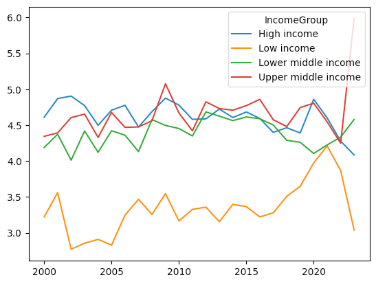
We can see a very sharp increase for the upper-middle income countries, and a decent rise in the lower-middle income countries. And we can see a steep drop among low-income countries. The big surprise to me was the drop in high-income countries, though. All countries changed around 2020, so part of me wonders whether some of it was pandemic-related... but I'm not sure.
That's it for this week's questions. My Jupyter notebook is here: https://drive.google.com/file/d/1dtvbFL-Jjm22H6JkIP9XzmwqDY0Ngvo2/view?usp=sharing
I'll be back next week with more data-analysis puzzles based on current events.
Reuven