


I’m writing this on my return flight from New York to Israel, finishing up 2.5 weeks in United States — attending PyCon, meeting with clients, and even getting a chance to see some family. The weather has been pretty warm. The weather awaiting me back in Israel will be even warmer. And of course, we’re a few weeks before the summer solstice, so we’re soon going to learn (or remember) how hot things can get.
Hot weather isn’t just annoying; it can be downright dangerous. A recent New York Times article (https://www.nytimes.com/2024/05/25/climate/extreme-heat-biden-workplace.html?unlocked_article_code=1.vk0.ekJ8.Kg0h3dcMGz9d&smid=url-share) discussed the challenges that workers face as weather becomes increasingly hot.
The article cited a number of sources, one of which was from the National Weather Service (https://www.weather.gov/), which publishes statistics about various weather-related disasters and hazards:
https://www.weather.gov/hazstat/
Data and seven questions
This week, I asked you to download a document from the National Weather Service summarizing the last 80 years of weather-related fatalities and damage in the United States:
https://www.weather.gov/media/hazstat/80years_2023.pdf
As you can see from the file extension, it's a PDF file. You'll want to use the Tabula-py (https://tabula-py.readthedocs.io/en/latest/) package to read this into Pandas.
This week, I asked you to answer seven tasks and questions. My solutions are below; a link to the Jupyter notebook I used to solve the problems myself follows the solutions.
The questions:
Download the PDF file describing extreme weather incidents. Read the table into a data frame. We don't need the final "All Wx Fatalities" column. We also don't need the final three rows with summaries and totals. Ensure that both header rows are used for the header names. How much memory is being used? What dtypes are being used?
I started off, as usual, by importing Pandas:
import pandas as pdBut because I want to grab data from a PDF file, I’ll use the “tabula-py” package. Specifically, I’ll use its “read_pdf” method. I’ll also define a “filename” variable that refers to the PDF file we downloaded:
from tabula import read_pdf
filename = '/Users/reuven/Downloads/80years_2023.pdf'
With these in place, we can now use “read_pdf” to create a data frame:
df = (
    read_pdf(filename,
             pages=1,
            multiple_tables=False,
             pandas_options={'header':[0,1]}
            )
    [0]
    .drop('All Wx', level=0, axis='columns')
    .iloc[:-3]
)
This works, but there are numerous problems with the HTML that we got:
- We get a warning that we didn’t specify the page we want.
- We didn’t explicitly indicate that there will only be one table on the page.
- The first row is taken to be the header, but it’s actually a two-line header
- We don’t need the “All Wx” column
- We don’t need the final three lines
How can I take care of these issues? Let’s handle them, one at a time. Thanks to method chaining, we can just add to our query, little by little.
First, let’s tell “read_pdf” that we only want to look on a single page, that there’s only one table, and that the header should come from both lines 0 and of the table. We can do this by passing several keyword arguments to “read_pdf”: “pages=1” tells it to only look on page 1, and “multiple_tables=False” tells is that there is one table.
But how can we tell “read_pdf” that we want to treat lines 0 and 1 as headers? That’s the sort of thing we would normally pass to “read_csv”, a Pandas method that we use all of the time. Does “read_pdf” take the same argument?
Not exactly: It doesn’t directly let us specify the header lines. But it does let us pass a keyword argument, “pandas_options”, whose value is a dict. Each key-value pair in that dict represents an option that we want to pass to “read_csv”, which is apparently invoked behind the scenes by “read_pdf”. So we can call:
df = (
    read_pdf(filename,
             pages=1,
            multiple_tables=False,
             pandas_options={'header':[0,1]}
            )
)
The result of calling “read_pdf” in this way isn’t a data frame. Rather, it’s a list of data frames. We only want one, and it’s the first one, so we’ll use “[0]” to retrieve the first element of that list:
df = (
    read_pdf(filename,
             pages=1,
            multiple_tables=False,
             pandas_options={'header':[0,1]}
            )
    [0]
)
Now let’s remove the “All Wx” column. It’s actually called “All Wx Fatalities”, but because we asked for two rows in our header, we now have a two-level multi-index. (We’ll fix that soon.) but I can invoke “drop”, indicating the name of the column I want to drop, as well as its level (0, indicating the outer part) and the axis (“columns”).
Remember that “drop” doesn’t modify the existing data frame, but rather returns a new one that lacks the dropped column(s):
df = (
    read_pdf(filename,
             pages=1,
            multiple_tables=False,
             pandas_options={'header':[0,1]}
            )
    [0]
    .drop('All Wx', level=0, axis='columns')
)
The only remaining issue, for now, is that the final three lines of the data frame contain totals and summaries that we don’t want to keep around. We can remove them by using “.iloc” to return all but the final three rows:
df = (
    read_pdf(filename,
             pages=1,
            multiple_tables=False,
             pandas_options={'header':[0,1]}
            )
    [0]
    .drop('All Wx', level=0, axis='columns')
    .iloc[:-3]
    .dropna(thresh=4)
)
Notice that I also invoked “dropna” to remove any row containing NaN values. That’s because I found that a row containing nothing but NaNs somehow got into the data frame when I imported it. By default, “dropna” removes any row containing even one NaN value. That’s too strict for our purposes, so I used the “thresh” keyword argument to say that as long as we have at least 4 good values, we should keep the row.
The end result is a data frame containing 84 rows and 11 columns. That’s fine, except that we have a very strange multi-index of column names; they are simply spread across two lines.
How can we make the column names a bit more normal?
My first thought was just to assign a list of strings back to “df.columns”. That will work, but it felt a bit of a cop-out. Surely there must be some way to just combine the two parts of the index into one.
If you look at a multi-index (i.e., just retrieve “df.columns”), you’ll see that it is basically a list of tuples. Yes, it’s a special Pandas object, and there are a number of ways to access it — but it’s easier in some ways to think of it as a list of tuples.
Since I know that each tuple contains two strings (from the outer and inner levels), maybe I can just iterate over each tuple, join the two parts together, and assign that to “df.columns”? Here’s how that would look:
df.columns = [' '.join(one_t)
             for one_t in df.columns]
This actually works! However, because the first column had a value for the outer layer and no value for the inner layer, Pandas provided one, “Unnamed: 0_level_1”. Which means that after running this comprehension, the first column has a name of “Year Unnamed: 0_level_1“. Not wrong, but not exactly what I would want.
I thus want to join the two parts of the tuple together unless the second part begins with “Unnamed”. In such a case, I’ll just take the first part. That sounds like an “if” statement in Python, but we can’t really put “if” statements, or any other statements, in list comprehensions. We can only include expressions.
One option would be to write a function, and then have that function include more complex logic, including “if” statements. The function could then return a string based on one or both tuple elements.
But this is one of those times when even I think it’s appropriate to use the expression version of “if-else” in Python. I generally avoid it, because I find it hard to read and understand. But it’s meant for precisely these situations. It syntax is
VALUE_IF_TRUE if CONDITION else VALUE_IF_FALSEThis is often compared with the “trinary” operator in C-like languages, aka ?: . The “trinary” name comes from the fact that it takes three arguments, as opposed to unary and binary operator, and doesn’t really describe what it does. It’s not quite the same, but it’s close. I even did a YouTube video about it:
Here, we can use it in this way:
df.columns = [one_t[0]
                if one_t[1].startswith('Unnamed')
                else ' '.join(one_t)
             for one_t in df.columns]
Having done this, I can now change the “Year” column to be an integer. (It was an “object” column before, because it contained a NaN value. Now that we’ve removed those and normalized the names, we can more easily change it.)
df['Year'] = df['Year'].astype('int16')After running the above code, I now have a data frame containing the data from the PDF file. What dtypes does it use? Let’s check, by grabbing the value of “dtypes” from the data frame:
Year                        int16
Lightning Fatalities      float64
Tornado Fatalities        float64
Flood Fatalities          float64
Hurricane Fatalities      float64
Heat Fatalities            object
Cold Fatalities           float64
Winter Fatalities         float64
Rip Curr. Fatalities      float64
Wind Fatalities           float64
All Hazard Damages (M)     object
dtype: object
How much memory does it use? Let’s check, using “memory_usage”. We specify “deep” to make sure that we could the size of each string object that is in Python memory, and thus not immediately available to Pandas:
df.memory_usage(deep=True).sum()I get the following back:
13293Not a crazy-huge value, but something to compare with.
Set all columns to be of type `pd.Int16Dtype` except for where `pd.Float64Dtype` or `pd.StringDtype` would be more appropriate. Remove any rows containing only NA values. Set "Year" to be the index. How much memory (if any) do you save by using these dtypes?
People are often surprised to find that NaN is a float value. This is annoying and weird if we have NaN in an integer column, because now the column must have a float dtype. But it often means that we need to give the column a dtype of “object”, in order to accommodate the different object types. That’s quite generic, and to some degree removes the usefulness of types in enforcing values and guaranteeing that methods will work.
We’ve talked about PyArrow in the past; one of its advantages over using NumPy is that it supports “nullable types.” In other words, you can have a string column that contains the equivalent of NaN, and it’ll stay a string column. You can have an integer column that contains the equivalent of NaN, and it’ll stay an int column. I say “the equivalent of NaN” because we don’t use NaN in this situation. Rather, we use “pd.NA”, a distinct Pandas-specific value that has the same idea as NaN, but works with these nullable types. NA is the reason why we have methods like “isna” as well as “isnan”, and keyword arguments like “skipna”.
Even if you’re not using PyArrow, Pandas provides us with built-in nullable types. These are known as “extension types,” and they have names like “pd.Int64Dtype”. The difference between extension types and regular Pandas types is that these use pd.NA rather than np.nan. In other words, they are nullable.
I asked you to change the dtypes for all columns to their equivalent extension types, and then to compare memory usage.
We can change the type of a column, as we saw before, with “astype”. That’s the typical way we do it; we take a column, run “astype” on it, indicate what dtype we want to get back, and then assign it back to the original column.
But there’s also a data frame version of “astype”, allowing us to convert many columns to new types. In this case, we indicate the new, destination types in a dict, with the column names as the keys and the new types as the values.
I decided that it would make sense to create such a dict using a dict comprehension. After all, we can iterate over each column name, and then provide an extension type as the value. But wait — what extension type should we provide? In most cases, as I indicated in the question, we’ll use “pd.Int16Dtype”. That should work for all columns except for one, “All Hazard Damages (M)”, which should use “pd.Float64Dtype”.
I decided that this would be a good place to use a dictionary. (Yes, this would be the second dictionary. The first one will be passed to “astype”. This one will be used to build the “astype” dict.) The dict would indicate which columns would use Int16Dtype and which would use Float64Dtype. But that seems like a lot of work, creating a dict with each column name.
I thus decided to use Python’s “defaultdict”. The default value we’ll return for our dict is pd.Int16Dtype. But if someone wants to use something else? That’s totally fine. Here’s how I created it:
from collections import defaultdict
conversion_dtypes = defaultdict(pd.Int16Dtype)
conversion_dtypes['All Hazard Damages (M)'] = pd.Float64Dtype()
The above means that I can now retrieve any key I want from “conversion_dtypes”. If I retrieve “All Hazard Damages (M)”, then I’ll get an instance of pd.Float64Dtype. Anything else? I’ll get an instance of pd.Int16Dtype. And yes, you need to invoke the extension type class in order to get an instance of it. It feels weird at first, but don’t worry — it feels weird later on, too.
Two of the columns contain commas and dollar signs. I used regular expressions and “str.replace” to handle them:
df['Heat Fatalities'] = (df
                         ['Heat Fatalities']
                         .str.replace(r'\D', '',
                                      regex=True)
                        )

df['All Hazard Damages (M)'] = (df
                                ['All Hazard Damages (M)']
                                .str.replace(r'[^\d.]', '',
                                             regex=True)
                               )
In the first regular expression, I asked to replace \D (i.e., any non-digit character) with the empty string. That took care of commas, allowing us to have integers in the column.
At first, I did the same thing for the second regular expression. But then I realized that I had removed the decimal points, which multiplied all of the values by 100. Whoops! I thus constructed a new regular expression, one using a “negative character class” — meaning that we’re looking for any character that isn’t a digit (\d) or a decimal point (.). Any non-digit, non-decimal point is replaced with the empty string.
With this in place, we can create our “conversions” dict, using a dict comprehension:
conversions = {column_name: conversion_dtypes[column_name]
              for column_name in df.columns}
The above dict has column names as keys and the extension types as values.
I had already removed the NaN-only row in the previous solution, so I was just left to perform the conversions and set “Year” to be our index:
df = (
    df
    .astype(conversions)
    .set_index('Year')
)
Sure enough, we can see that I’m using extension types:
Lightning Fatalities        Int16
Tornado Fatalities          Int16
Flood Fatalities            Int16
Hurricane Fatalities        Int16
Heat Fatalities             Int16
Cold Fatalities             Int16
Winter Fatalities           Int16
Rip Curr. Fatalities        Int16
Wind Fatalities             Int16
All Hazard Damages (M)    Float64
dtype: object
It’s sometimes hard to see, but notice that each extension type name is capitalized, as is traditional with Python class names.
Did this save us any memory? I again run
df.memory_usage(deep=True).sum()And I get
3276In other words, we’re using about one third the memory of the NumPy value equivalents. And we can now use pd.NA, which is more elegant.
What is the first year in which each measurement was taken?
Looking at the table with our eyes, we can see that the National Weather Service started to collect data about four hazards in 1940, but added others only later. I wanted to know when each hazard started to be measured.
I’d like to find out the year in which each column was first measured. Another way to describe this is that for each column, I want to get the first non-NA value. How can I do this?
There actually is a Pandas function that can help! The “first_valid_index” method for a series returns the index for the first non-NA value. Given that our index now contains years, this seems perfect for our purposes.
The thing is, we want to invoke “first_valid_index” on each column. To do that, we’ll use the “apply” method for data frames, which allows us to invoke a function on each column:
df.apply(lambda col: col.first_valid_index())Notice that “first_valid_index” is a series method. We must thus invoke it on a column. We use a “lambda” expression to capture each column, one at a time, in the data frame, via the “col” parameter. We can then invoke “first_valid_index” on each column. The result we get back:
Lightning Fatalities      1940
Tornado Fatalities        1940
Flood Fatalities          1940
Hurricane Fatalities      1940
Heat Fatalities           1986
Cold Fatalities           1988
Winter Fatalities         1986
Rip Curr. Fatalities      2002
Wind Fatalities           1995
All Hazard Damages (M)    1988
dtype: int16
As a general rule, any method you can run on a series can also run on a data frame, and we’ll get back one value for each column. There is a “first_valid_index” method for data frames, as well — couldn’t we just invoke that, instead of using “apply”?
Sadly, the answer is “no,” because “first_valid_index” on a data frame returns the first index for which there is at least one non-NA value in the data frame. In other words, invoking “df.first_valid_index()” would return the integer 1940.
The New York Times story says that "heat kills more people each year than hurricanes, floods and tornadoes combined." Does this match the data we have? Show it both numerically and in a bar graph, comparing on an annual basis.
To answer this question, we’ll need to create a new column — albeit temporarily — that combines the fatalities from hurricanes, floods, and tornadoes. We can do this most easily with “assign”, whose keyword arguments indicate what new columns we want, and the values we want to assign to them. Invoking “assign” returns a new data frame with the specified column(s) in it, but doesn’t change the original data frame.
I can get the new column, which I called “hur_flo_tor” in order to confuse the next person who will work on this project, in the following way:
(
    df
    .assign(hur_flo_tor=lambda df_: (df_['Hurricane Fatalities'] +
                                     df_['Flood Fatalities'] +
                                     df_['Tornado Fatalities']))
)
I only care about two columns, “hur_flo_tor” and our original “Heat Fatalities” column. We can select a single column with [], and to get a list of columns, we put a list of strings inside. I also remove any rows in which we have NA values; that won’t help us make any comparisons:
(
    df
    .assign(hur_flo_tor=lambda df_: (df_['Hurricane Fatalities'] +
                                     df_['Flood Fatalities'] +
                                     df_['Tornado Fatalities']))
    [['hur_flo_tor', 'Heat Fatalities']]
    .dropna()
)
The result:
      hur_flo_tor  Heat Fatalities
Year
1986          120               40
1987          129               38
1988           72               41
1989          173                6
1990          195               32
1991          119               36
1992          128                8
1993          138               20
1994          169               29
1995          127             1021
1996          193               36
1997          186               81
1998          275              173
1999          181              502
2000           79              158
2001          112              166
2002          155              167
2003          154               36
2004          151                6
2005         1097              158
2006          143              253
2007          169              105
2008          220               71
2009           79               45
2010          148              138
2011          675              206
2012          102              156
2013          138               92
2014           87               20
2015          237               45
2016          155               94
2017          178              107
2018           97              108
2019          134              187
2020          157              350
2021          262              375
2022          232              383
2023          159              207
A quick look at these numbers makes it seem that actually, the NYT story was accurate: Over the last few years, more people have died as a result of extreme heat than from hurricanes, floods, and tornadoes combined.
We can create a bar graph from this data, by invoking “plot.bar”:
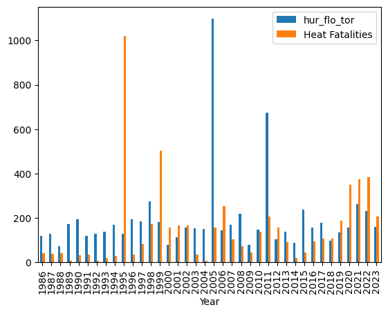
The graph shows that yes, there were years in which heat fatalities were lower than hurricanes, floods, and tornadoes combined — but they are rare, especially as time has marched forward.
What is the percentage year-over-year change in heat-related deaths? Do we see them increasing in the last few years?
To calculate this, I first grabbed the “Heat Fatalities” column from the data frame:
(
    df
    ['Heat Fatalities']
)
I then ran “pct_change” , a convenient window function that returns a new series indicating (as you would expect) the percentage change that each row’s value reflects from the previous one. The returned series has the same index as the original. The first row is always NA, because it has no predecessor; in our case, we’ll have a lot of NA values, because measurements didn’t start in the first year of the data frame. We can remove them with “dropna”:
(
    df
    ['Heat Fatalities']
    .pct_change()
    .dropna()
)
I then asked you to find if we had seen an increase in heat-related deaths in recent years. I didn’t define “recent”, but I’ll take it to mean 20. I use “tail” to get the 20 most recent values:
(
    df
    ['Heat Fatalities']
    .pct_change()
    .dropna()
    .tail(20)
)
Now I want to know whether the values were increasing (i.e., a positive percentage) or decreasing (i.e., a negative percentage). I’ll use the “gt” method, which implements the “>” operator and returns True/False values for each element in our series:
(
    df
    ['Heat Fatalities']
    .pct_change()
    .dropna()
    .tail(20)
    .gt(0)
)
Finally, I use “value_counts” to count the number of times we have True/False values:
(
    df
    ['Heat Fatalities']
    .pct_change()
    .dropna()
    .tail(20)
    .gt(0)
    .value_counts()
)
The result:
Heat Fatalities
True     12
False     8
Name: count, dtype: Int64
In other words, in 12 of the last 20 years, we saw an increase in heat-related deaths from the previous year. That’s not a perfect measure, especially because it doesn’t take the magnitude of the change into account, but it does show that overall, heat-related deaths are growing in number.
With which other weather-related fatality types do we see the strongest correlation with heat fatalities? Is that a strong correlation?
It’s often useful to find correlations between different columns. That is: When one value goes up, does another value go up proportionally? If so, that’s a positive correlation; we can measure it between 0 (none) and 1 (complete). Or when a value goes up, does another value go down proportionally? If so, that’s a negative correlation, which we measure between 0 (none) and -1 (complete). A positive correlation of 0.8 is very strong, and one of 0.2 is pretty weak.
We can run the “corr” method on our data frame to find correlations across all of our columns. We’ll get back a data frame, showing each piece of information twice. I’ll thus start by running “corr” and then immediately grabbing only the “Heat Fatalities” column:
(
    df
    .corr()
    ['Heat Fatalities']
)
The “corr” method calculates correlations across all columns, including themselves — which are, by definition, correlated at 100%, or 1. We can remove the self-correlation row from our series, as well as that for “All Hazard Damages”, which is showing monetary damages, not human lives lost:
(
    df
    .corr()
    ['Heat Fatalities']
    .drop(['Heat Fatalities', 'All Hazard Damages (M)'])
)
I can then take the remaining values in the series and sort them with “sort_values”:
(
    df
    .corr()
    ['Heat Fatalities']
    .drop(['Heat Fatalities', 'All Hazard Damages (M)'])
    .sort_values(ascending=False)
)
Here’s what I get:
Rip Curr. Fatalities    0.438377
Wind Fatalities         0.324180
Tornado Fatalities      0.091718
Hurricane Fatalities    0.032445
Lightning Fatalities    0.023165
Flood Fatalities       -0.047615
Cold Fatalities        -0.147345
Winter Fatalities      -0.227027
Name: Heat Fatalities, dtype: float64
We see a semi-strong positive correlation with rip current fatalities and wind fatalities, but they aren’t super strong. The rest are either very weak or negative. Indeed, we see a strong negative correlation with winter facilities, which makes sense — in years where there are many heat deaths, we would expect fewer winter-related deaths, and vice versa, just because of the warmth (or not) of that year’s weather.
How much, in millions of dollars, is the damage due to weather-related incidents? Create a line plot showing that amount. Can you think of what the peaks might represent?
We can plot annual damage with “plot.line”:
df['All Hazard Damages (M)'].plot.line()Note that this works because our index was previously set to the years. Years will thus be our x axis, and the y axis will be the value, in millions of dollars, of damage done by these hazards:
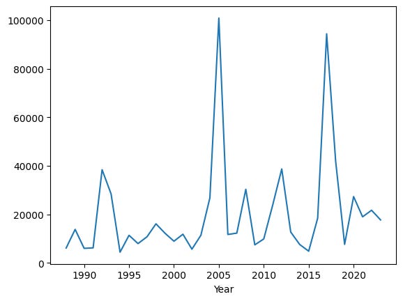
The biggest values are in 2005, 2017, 2018, and 2012. What happened in each of those years? I’m not sure, but from a quick look at Wikipedia (https://en.wikipedia.org/wiki/List_of_natural_disasters_in_the_United_States), I see that 2005 had hurricane Katrina, and 2017 had both wildfires and hurricane Maria. So these make sense, even if they’re rather grim.
You can download my Jupyter notebook from here: https://drive.google.com/file/d/1kbCA9BKtq43mn9_AnGhWYFhWjtMfq0JT/view?usp=sharing
I’ll be back next week with more Pandas challenges!
Reuven