


Reminder: My latest HOPPy (Hands-On Projects in Python) course, where you design and build your own game using agentic coding, starts on Sunday! I can't think of any better way to level up your skills, as well as have a project in your portfolio. Learn more at https://LernerPython.com/hoppy .
AI continues to dominate the news headlines. And with US midterm elections coming up, one topic has been in the headlines quite a bit, namely the number of data centers currently being planned and built. These data centers are often massive – with at least one reported to be the size of Manhattan – and local residents in many states have indicated that they don't want this sort of thing nearby.
The politics of data centers are crossing party lines, too, with Governor Josh Shapiro of Pennsylvania (a Democrat) and Governor Greg Abbott of Texas (a Republican) both backtracking from their previously enthusiastic endorsements of data-center construction.
Meanwhile, Donald Trump is all in on data centers, saying that anyone who doesn't want them is stupid and wants to be poor – a political argument that The Bulwark recently described as so tone deaf, "Next, we suspect he will launch into caps-lock tirades against ice cream, puppies, and the Beatles" (https://www.thebulwark.com/p/donald-trump-ai-hubris-is-a-blue-democratic-opportunity).
Meanwhile, Republican politicians are struggling to find a way to please both Trump and their constituents (https://www.nytimes.com/2026/09/29/us/republicans-trump-data-center-ai.html?unlocked_article_code=1.FFE.1X-0.AanfR5azyTjm&smid=url-share).
This week, we'll look at when and where data centers are being built. But there's a catch: We'll do it not writing the Pandas queries ourselves, but instead during it using agentic coding. (I'm partial to Claude Code, but you can use any agentic coding system you want, using any models you want.) The idea is that we'll pose questions to the agents and ask for analysis from them – with the output going into a Marimo (or Jupyter) notebook. Then we can look at their queries, and see if we can learn something.
This week's questions are deliberately harder than usual, because I'm assuming you'll ask agents to do the hard work for you.
Data and five questions
There are a number of data sources, none of them perfectly authoritative, that you (or your AI agent) might wish to use, including:
- Epoch: https://epoch.ai/data/ai-data-centers
- FracTracker: https://fractracker.org/2026/04/open-u-s-data-centers-tracker/
- Interconnection: https://www.interconnection.fyi/data-center
Paid subscribers, both to Bamboo Weekly and to my LernerPython+data membership program (https://LernerPython.com) get all of the questions and answers, as well as downloadable data files, downloadable versions of my notebooks, one-click access to my notebooks, and invitations to monthly office hours.
Learning goals for this week include: Using agentic coding to perform data analysis — and then understanding the techniques it used.
Here are the solutions and explanations for this week's five questions:
Retrieve data from one or more of the above sources (or others, if you know of them), combining them into a single Pandas data frame. Keep only data about the United States. Using Plotly, create a bar plot showing the number of data centers in the United States each year.
One of the things I love about using agents is that they come up with ideas that I never would have imagined. Sometimes, those ideas are great ones, in which case it's like a super-successful brainstorming session. Sometimes those ideas are real lemons, which is why it's important to have your finger on the pulse of what the agents are doing.
I gave Claude Code the introduction to this week's questions, and also the questions themselves. I didn't give it anything beyond that, and was curious to see what it would do. I did, however, ask it to produce the output in a Marimo notebook.
It would seem that it looked around the directory in which I produce Bamboo Weekly and decided to mimic the way that I've done things for a while — including both putting all of the import statements in one cell at the top of the notebook, and putting data files under the data subdirectory, with files named bw-xxx-name, where xxx is the issue number for which it's relevant.
It thus started with a huge number of import statements, far more than I would have done myself:
import pandas as pd
from pandas import Series, DataFrame
from plotly import express as px
import bson
import io
import os
import urllib.request
import numpy as np
import requests
from scipy import stats
from plotly import graph_objects as go
from plotly.subplots import make_subplots
I mean....how many of these do we really need? A giveaway clue was the import bson statement. Do I really need to load bson? And if so, then why? I have a feeling that Claude Code decided to import the union of all (or most) modules that are mentioned in any and all of my other (previous issues') Bamboo Weekly notebooks. This is... a silly way to go, to say the least. It doesn't hurt, but it does take more time and memory, wasting it on unnecessary packages.
Claude then created a dictionary with the CSV data from each of the sources that I had mentioned. The idea was to download each of them, one by one, from their web sites, putting them into files.
I didn't instruct Claude regarding where to store these files – but it looked around, and saw that previous issues' data files were in the "data" subdirectory under my notebooks, each with "bw-nnn" at the start of the filename, indicating the issue for which it was relevant. Here is the mapping from filenames to URLs/sources:
_downloads = {
    'data/bw-190-epoch-data_centers.csv': 'https://epoch.ai/data/data_centers/data_centers.csv',
    'data/bw-190-epoch-data_center_timelines.csv': 'https://epoch.ai/data/data_centers/data_center_timelines.csv',
    'data/bw-190-census-states.txt': 'https://www2.census.gov/geo/docs/reference/state.txt',
    'data/bw-190-census-pop-2025.csv': 'https://www2.census.gov/programs-surveys/popest/datasets/2020-2025/state/totals/NST-EST2025-ALLDATA.csv',
    'data/bw-190-census-income-h08.xlsx': 'https://www2.census.gov/programs-surveys/cps/tables/time-series/historical-income-households/h08.xlsx',
    'data/bw-190-census-gazetteer-2024.zip': 'https://www2.census.gov/geo/docs/maps-data/data/gazetteer/2024_Gazetteer/2024_Gaz_state_national.zip',
    # EIA-860M lags ~2 months; August 2026 is the newest real file as of 2026-09-30
    'data/bw-190-eia860m-august-2026.xlsx': 'https://www.eia.gov/electricity/data/eia860m/xls/august_generator2026.xlsx',
}

for _filename, _url in _downloads.items():
    if not os.path.exists(_filename):
        urllib.request.urlretrieve(_url, _filename)
You can then see that Claude asked Python to iterate over the dictionary, retrieving each URL into the specified file. I haven't ever done this before, but it's not a bad technique – I might use this in the future!
Before creating a data frame based on these downloaded files, Claude also downloaded Census data about the 50 US states. That not only provides state names and abbreviations, but also makes it possible (as Claude's comments point out) to easily do a join on the other data files, keeping only US data:
states_df = (
    pd.read_csv('data/bw-190-census-states.txt', sep='|', dtype=str)
    .loc[pd.col('STATE').astype(int) <= 56]
    .rename(columns={'STATE': 'fips', 'STUSAB': 'state', 'STATE_NAME': 'state_name'})
    [['fips', 'state', 'state_name']]
)
But of course, all this just downloaded the data. It didn't create a data frame. To do so, Claude had to download data from three sources, then combine them.
For example, here's how it handled the Interconnection data: It checked to see if the output file doesn't yet exist, saving us time and energy creating the file. It then read the HTTP response into read_html, which returns a list of data frames, one for each HTML table on the page. It then iterated through each state in states_df, using it to retrieve data about that particular state. It used assign to add a state column in each with the state's name.
The result was a list of per-state data frames, which were then combined together with pd.concat. That was then written to a parquet-format file before being read back into interconnection_df. This ensures that we not only have the data in memory, but also on disk if we need to recreate it:
_filename = 'data/bw-190-interconnection.parquet'

if not os.path.exists(_filename):
    (
        pd.concat([pd.read_html(io.StringIO(_response.text))[0].assign(state=_state)
                   for _state in states_df['state']
                   if (_response := requests.get(f'https://www.interconnection.fyi/data-center/state/{_state}')).ok],
                  ignore_index=True)
        .to_parquet(_filename)
    )

interconnection_df = pd.read_parquet(_filename)
For the second data source, Claude did something similar:
_filename = 'data/bw-190-fractracker.parquet'
_url = 'https://services.arcgis.com/jDGuO8tYggdCCnUJ/arcgis/rest/services/data_centers_v4_agol_all/FeatureServer/0/query'

if not os.path.exists(_filename):
    _count = requests.get(_url, params={'where': '1=1', 'returnCountOnly': 'true', 'f': 'json'}).json()['count']
    (
        pd.concat([DataFrame(Series(requests.get(_url, params={'where': '1=1', 'outFields': '*', 'f': 'json',
                                                               'resultOffset': _offset, 'resultRecordCount': 1000})
                                    .json()['features'])
                             .str['attributes'].tolist())
                   for _offset in range(0, _count, 1000)],
                  ignore_index=True)
        .to_parquet(_filename)
    )

fractracker_df = pd.read_parquet(_filename)
The big difference with Fractracker was that the URL needed to retrieve each part of the data was more complex, with more parameters. I'll note that I didn't give any hints regarding how it should download the data, or what tools it should use. However, using the requests library seems more than reasonable.
The Epoch data was by far the most complex, but also included construction timelines, which we had already read into a CSV file:
epoch_timelines_df = (
    pd.read_csv('data/bw-190-epoch-data_center_timelines.csv', engine='pyarrow')
    .assign(Date = pd.col('Date').pipe(pd.to_datetime))
)
Claude then got the state names from states_df, partly in order to handle mailing addresses with state names and/or abbreviations:
_state_names = (
    states_df
    .assign(name_length = pd.col('state_name').str.len())
    .sort_values('name_length', ascending=False)     # "West Virginia" before "Virginia"
    ['state_name']
    .str.cat(sep='|')
)
Then came a huge method chain, the type that often throws people off:
epoch_df = (
    pd.read_csv('data/bw-190-epoch-data_centers.csv', engine='pyarrow')
    .loc[pd.col('Country') == 'United States']
    .assign(
        postal = pd.col('Address').str.extract(r'\b([A-Z]{2})[,\s]+\d{5}')[0]         # "..., TN 38109, USA"
                 .fillna(pd.col('Address').str.extract(r',\s*([A-Z]{2})\s*$')[0]),  # "..., The Dalles, OR"
        name_state = (pd.col('Name') + ' ' + pd.col('Address').fillna(''))
                     .str.extract(f'({_state_names})(?! City)')[0]
                     .map(states_df.set_index('state_name')['state']),
        state = pd.col('postal').where(pd.col('postal').isin(states_df['state'])).fillna(pd.col('name_state')),
        owner = pd.col('Owner').str.replace(r'\s*#\w+', '', regex=True),   # drop Epoch's "#confident" tags
        first_operational = pd.col('Name').map(
            epoch_timelines_df
            .loc[pd.col('Buildings operational') > 0]
            .groupby('Data center')['Date'].min()),
    )
)
Here's what happened in the above code:
- It read the Epoch data-center info into a data frame with
read_csv. - It used
locandpd.colto keep only rows from the United States. - It assigned three new columns:
postal, the postal address, including the statename_state, the name of the state from the addressstate, the actual stateowner, the owner of the data center, andfirst_operational, adatetimevalue indicating when the data center went online.
Note that it uses where, something that I've almost never used in my own queries, but probably should do more of.
With these three data frames in memory, we then had to join them together. This is a pretty common problem, and we've dealt with it in many previous Bamboo Weekly editions. Typically, you can either use join to combine along the index or merge to combine arbitrary columns.
But there's another way, using pd.concat. It does a form of join as well, even if we don't think of it in that way. The only catch is that all of the data frames we hand to pd.concat need the same columns to join vertically, or rows to join horizontally. (The latter is basically a join.)
Claude took each of the three data frames it had already created, use assign to create new columns that would match up, and then combined them. The result was dc_df, a data frame with 5,632 rows and 8 columns, each representing one data point. The source column in dc_df indicated where the data had come from:
_status_order = ['operating', 'expanding', 'under construction', 'proposed', 'cancelled/suspended', 'unknown']

dc_df = (
    pd.concat([
        interconnection_df
        .assign(source = 'Interconnection.fyi',
                name = pd.col('Facility Name'),
                status = pd.col('Status').map({'Operational': 'operating', 'Construction': 'under construction',
                                               'Proposed': 'proposed', 'Cancelled': 'cancelled/suspended',
                                               'Unknown': 'unknown'}),
                capacity = pd.col('Capacity').replace('—', None)),

        fractracker_df
        .assign(source = 'FracTracker',
                name = pd.col('facility_name'),
                state = pd.col('state').str.strip(),
                operator = pd.col('operator_name').str.strip().replace('', None),
                status = pd.col('status').map({'Operating': 'operating', 'Expanding': 'expanding',
                                               'Approved/Permitted/Under construction': 'under construction',
                                               'Proposed': 'proposed', 'Pre-proposal': 'proposed',
                                               'Cancelled': 'cancelled/suspended', 'Suspended': 'cancelled/suspended'}),
                mw = (pd.col('mw_low') + pd.col('mw_high')) / 2,
                year = pd.col('expected_date_online').str.extract(r'(20[2-4]\d)')[0].astype(float)),

        epoch_df
        .assign(source = 'Epoch AI',
                name = pd.col('Name'),
                operator = pd.col('owner'),
                status = pd.col('first_operational')
                         .le(pd.Timestamp.today())
                         .map({True: 'operating', False: 'under construction'}),
                mw = pd.col('Current power (MW)'),
                year = pd.col('first_operational').dt.year),
    ], ignore_index=True)
    .loc[pd.col('state').isin(states_df['state'])]
    [['source', 'name', 'state', 'operator', 'status', 'mw', 'capacity', 'year']]
    .astype({'source': 'category', 'state': 'category', 'operator': 'category', 'capacity': 'category',
             'status': pd.CategoricalDtype(_status_order, ordered=True),
             'mw': 'float32', 'year': 'Int16'})
    .reset_index(drop=True)
)
To its credit, Claude then added what it called a "sanity check" query, making sure that the number of rows from each source matched the original data:
pd.concat([
    pd.Series({'Interconnection.fyi': len(interconnection_df), 'FracTracker': len(fractracker_df),
               'Epoch AI': len(epoch_df)}, name='loaded (US)'),
    dc_df['source'].value_counts().rename('kept'),
    dc_df.groupby('source', observed=True)['year'].count().rename('with year'),
    dc_df.groupby('source', observed=True)['state'].count().rename('with state'),
    dc_df.pivot_table(index='source', columns='status', values='name', aggfunc='count', observed=False),
], axis=1)
This is a pretty smart, quick check to ensure that you haven't lost any data. Notice that it used groupby on source with both year and state, double checking that all of the data had been captured along more than one axis.
It also, a bit to my surprise, used memory_usage to check how much memory was being used, which turned out to be laughably small, at 256 KB. (When was the last time you measured something in kilobytes?!?) That's largely thanks to the categories that Claude defined, turning each of the strings into a small integer.
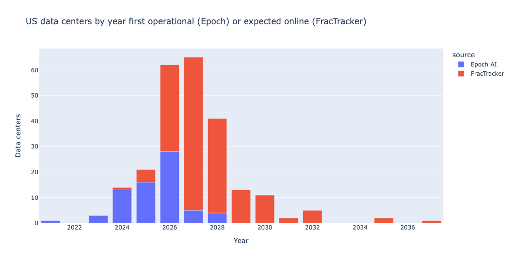
I then asked for a Plotly bar graph, showing how many data centers are being constructed in each year.
Claude's query grabbed all of the rows with non-NaN years and non-cancelled/suspended status. It then ran groupby on the year and source. It then used pipe to invoke px.bar, passing a number of keyword arguments to make the plot a bit easier to read:
(
    dc_df
    .loc[pd.col('year').notna() & (pd.col('status') != 'cancelled/suspended')]
    .groupby(['year', 'source'], observed=True)
    .size()
    .reset_index(name='data_centers')
    .pipe(px.bar, x='year', y='data_centers', color='source',
          title='US data centers by year first operational (Epoch) or expected online (FracTracker)',
          labels={'year': 'Year', 'data_centers': 'Data centers'})
)
I must admit that I didn't expect this year (i.e., 2026) to be close to the left side of the plot, with future construction already included – but I shouldn't have been surprised. That said, it's pretty clear why data centers are suddenly on everyone's minds – after a handful of data centers built every year for a while, the number jumped to 60 (!) in 2026, with even more planned for 2027, and over 40 already planned for 2028.
Here's the plot:
Using Plotly, create a bar plot showing (as of the most recent data) how many data centers there are per state. If you have data for it, use a stacked bar plot to break each state-count bar into pieces, showing how many centers are associated with each company.
How many data centers are there per state? Here, used a pretty reasonable set of queries:
- First, it used
locto keep only those data centers currently operating or expanding. However, it useddc_dfinside ofloc, something that I tell my students to avoid in favor oflambdaor (better yet, now that we can use Pandas 3)pd.col. - It then used
pivot_tableto turn the different states and sources into a data frame, counting the number of data centers per state, per source. - It then used
sort_valuesto get the 20 states with the most data centers, at least according to Interconnection.
(
    dc_df
    .loc[dc_df['status'].isin(['operating', 'expanding'])]
    .pivot_table(index='state', columns='source', values='name', aggfunc='count', observed=False)
    .sort_values('Interconnection.fyi', ascending=False)
    .head(20)
)
Here's what we see:
state	Epoch AI	FracTracker	Interconnection.fyi
TX	9	74	693
VA	7	214	602
CA	0	9	324
OR	2	11	296
AZ	1	10	77
IL	0	5	51
NJ	1	5	50
GA	3	87	47
CO	0	4	34
NM	1	5	21
NY	2	17	20
OH	4	20	18
WA	0	17	15
MD	0	3	15
MO	0	5	13
MA	0	2	13
UT	1	2	12
PA	1	42	11
IA	2	6	11
NE	4	6	11
I'm not surprised that Texas (#1) or California (#3) has a huge number of data centers, but I completely forgot how many are in Virginia – wow!
I then asked for stacked bar plots, breaking down the owner of each data center in each state. Claude kept the first part of the above query, but then used assign to create some additional columns (much as I would do!), and then ran groupby to get per-state and per-company data:
_top_operators = (
    dc_df
    .loc[pd.col('source') == 'FracTracker', 'operator']
    .value_counts()
    .head(12)
    .index
)

(
    dc_df
    .loc[(pd.col('source') == 'FracTracker') & (pd.col('status') != 'cancelled/suspended')]
    .assign(company = pd.col('operator').astype(str)
                      .where(pd.col('operator').isin(_top_operators), 'Other')
                      .where(pd.col('operator').notna(), 'Unknown'))
    .groupby(['state', 'company'], observed=True)
    .size()
    .reset_index(name='data_centers')
    .assign(state_total = pd.col('data_centers').groupby(pd.col('state')).transform('sum'))
    .sort_values(['state_total', 'data_centers'], ascending=False)
    .pipe(px.bar, x='state', y='data_centers', color='company',
          color_discrete_sequence=px.colors.qualitative.Dark24,
          color_discrete_map={'Other': 'lightgray', 'Unknown': 'darkgray'},
          title='Data centers (operating + in development) per state, by company -- FracTracker, Sept 2026',
          labels={'data_centers': 'Data centers', 'state': 'State'})
)
Here's the bar plot we got:
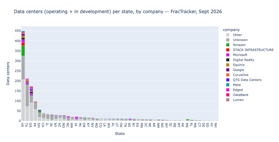
It's pretty astonishing to see how many data centers are in Virginia, and how many different companies are there. But to me, the most telling thing is how many data centers are listed as "Other" or "Unknown." Claude's notes indicate that in many cases, an operator runs a data center under a non-disclosure agreement, forbidding them from saying who it is for. Which ... might ruffle even more feathers, with big, anonymous companies building massive pieces of computing infrastructure.