


Two announcements:
- My advanced Claude Code workshop is happening on Wednesday, September 30th. Join me, as I share (via exercises and short projects) lots of details about building robust software systems with AI. You'll come away more prepared than ever to write apps with Claude Code. More info: https://lernerpython.com/code-with-claude/
- Want to play a game? How about write a game? Join my upcoming HOPPy (Hands-on Projects in Python) course, where we'll be using agentic coding to build a game — one that you design and specify. More info at https://lernerpython.com/hoppy/, or join a free info session about HOPPy 6 at https://us02web.zoom.us/meeting/register/JrZ8vOTgQX2CrOlULbQV2A .
Over the last few weeks, I've heard a lot about AI. One of the most common themes has been the dangers posed by AI, especially in the wake of various security incidents reported by companies like OpenAI and Anthropic, and the loud resignations of people worried about what AI might do to humanity. Casey Newton summarized many of these in his (really excellent) Platformer newsletter: https://www.platformer.news/ai-safety-vibe-shift-coxon-anthropic/
I thought it would thus be appropriate to take some time this week to examine data about AI safety, examining the timing, number, and types of incidents that have taken place.
Data and five questions
This week's data comes from the AI incident database (https://incidentdatabase.ai/). As you can probably understand from the name, the database contains information about thousands of incidents caused by, or with the help of, AI.
You can download a snapshot of the database from https://incidentdatabase.ai/research/snapshots/ . New snapshots are made available every Monday; we will be using the database from Monday, September 21st, 2026. The snapshot file contains data in a few different formats. I decided, for a variety of reasons, to use the BSON (https://en.wikipedia.org/wiki/BSON) formatted files. This format introduces a number of issues and wrinkles when importing them into Pandas. If you download the files yourself, you'll need to extract them from a bz2 archive. For our exercises, we'll only need incidents.bson and classifications.bson.
Paid subscribers, both to Bamboo Weekly and to my LernerPython+data membership program (https://LernerPython.com) get all of the questions and answers, as well as downloadable data files, downloadable versions of my notebooks, one-click access to my notebooks, and invitations to monthly office hours.
Learning goals for this week include: Reading BSON files, complex data, grouping, plotting, joins, and dates and times.
Here are the solutions and explanations for this week's five questions:
Load the incidents.bson file into a Pandas data frame. Make the "id" column into the index, and the "date" column have a datetime dtype. Create a line plot showing the number of incidents reported per day (as per the date column) in the database. Do you see any obvious trend?
First, I loaded up a few modules that I would need — Pandas and Plotly, as per usual. I also imported the name DataFrame from Pandas, so that I could use it without the pd. prefix. And I also installed (with uv) and imported bson from the pymongo (https://pypi.org/project/pymongo/) package on PyPI, which provides a bson module. Note that you don't want to download and install the bson package from PyPI, which won't work:
import pandas as pd
from pandas import DataFrame
from plotly import express as px
import bson
With those in place, we can read the BSON file into a data frame.
But wait: What is BSON? And how can we read it into a data frame?
In a nutshell, BSON is "Binary JSON" format, something that was created and popularized by MongoDB, the company behind one of the first and most famous "NoSQL" databases, aka a "document database." You can think of MongoDB as a database that works with Python dictionaries — or, as they're known in the JavaScript world, with "objects."
While JSON has become the lingua franca of APIs and Internet communication, it supports a limited set of data structures. It is also text-based, which means that it can take up a lot of space. BSON solves the former problem by including a large number of data types that aren't native to JSON, including booleans and datetimes. It solves the latter problem by being binary and compressed. So you can think of BSON as a second-generation JSON — smaller, faster, and more capable.
But whereas JSON is supported by the json module in Python's standard library, and can be turned from its textual format into Python objects with a simple call to json.loads, BSON requires a bit more work.
First, as I mentioned above, don't download the bson package from PyPI. Rather, download the pymongo package, and then import bson that it provides.
Still though, how can you read a BSON file into Python? And how can you then turn it into a data frame?
You can think of a BSON file as a being equivalent to a Python list of dictionaries. (Each dict is, again, equivalent to a JSON "object," or what the BSON world calls a "document.") As you might know, you can actually create a data frame by invoking DataFrame on a list of dictionaries. Each dict becomes one row in the data frame; the dict keys become the column names, and the dict values become the cells for that row. The assumption is that all of the dicts have the same (or similar) keys.
To get there, we'll need to read a BSON file into a list of dicts. We can do that by first opening the file in read-binary mode (since it isn't text), and then invoking the read method, returning the entirety of the file's contents.
Note: When teaching Python courses, I generally tell people not to just invoke the read method on a file, because it could potentially be such a large file that reading the whole thing into memory might blow up your program. But here, there's really no choice – and besides, the data frame will contain all of the file's data, so we'll need to read the whole thing somehow.
Once you've read the entire file, you pass it to bson.decode_all. That method returns the list of dicts that we want, which we can then pass to DataFrame. Here's what the code looks like, inside of a with block that automatically closes the file after we're done with it:
incidents_filename = 'data/bw-189-incidents.bson'

with open(incidents_filename, 'rb') as _f:
    incidents_df = (
        DataFrame(bson.decode_all(_f.read()))
    )
Now, the fact is that this will work – but there are two additional tasks we need to think about. First, we need to turn incident_id into the data frame's index. We can do that by invoking set_index. We also need to turn date, which is a string (and somehow not a real datetime value) into a datetime dtype. We can do that by invoking pd.to_datetime on the date column; here, I did it using a combination of assign, pd.col, and pipe as well as pd.to_datetime:
assignadds a new column to a data frame. It takes keyword arguments, where the keyword name is the new column name, and the value contains the valuepd.collets us retrieve one column by namepipelets us pretend that a function is actually a method, and thus keep the method chain going.
The combination, which gives us a new date column with datetime values, looks like this:
incidents_filename = 'data/bw-189-incidents.bson'

with open(incidents_filename, 'rb') as _f:
    incidents_df = (
        DataFrame(bson.decode_all(_f.read()))
        .set_index('incident_id')
        .assign(date = pd.col('date').pipe(pd.to_datetime))
    )
The result is a data frame with 1,691 rows and 24 columns.
I then asked you to create a line plot showing the number of reported incidents per year. Remember that the AI incident database gets reports from people around the world, and not everyone knows (or cares) to report incidents to them. Nevertheless, I wanted to see if the number of incidents has grown.
To do that, I first invoked reset_index, to move the index into a regular column. Then, to count the number of incidents per date, I invoked groupby, grouping on the date column, using the count aggregation method on the incident_id column. This gave me a series in which dates were the index and the number of incidents per date were the values. I then used pipe and px.line to create the plot:
(
    incidents_df
    .reset_index()
    .groupby('date')['incident_id'].count()
    .pipe(px.line)
)
The result:
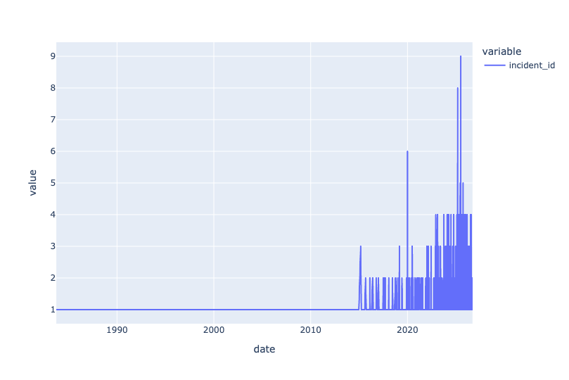
We can certainly see more incident reports in the last few years. But daily reports might make it a bit messy, so I decided to count them by month, using resample and asking for a frequency of 1ME, or the end of every one-month period:
(
    incidents_df
    .reset_index()
    .groupby('date')['incident_id'].count()
    .resample('1ME').sum()
    .pipe(px.line)
)
The result was a bit more dramatic:
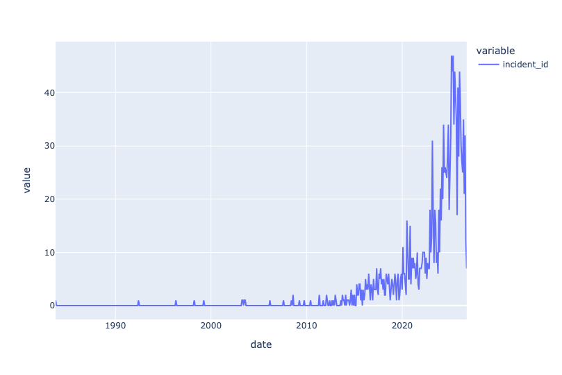
However, we also see a decline in the last year (i.e., since late 2025). Whether that's because of late reporting of incidents or the time it takes to process them, I'm not sure. But we're still seeing many more reports each month than was true just 10 years ago.
What were reported to be the 10 most common developers of these incidents? Who were the 10 most commonly harmed people in these incidents?
Our data set has a column, Alleged developer of AI system, which tells us who developed the problematic software.
You might think that we can then run value_counts on this column, and get the most common culprit. But that's not quite true, because the column contains lists of strings, not strings. To break those lists apart into separate elements, we can use explode. You can think of explode as a version of str.split; if a series contains one 3-element list and one 2-element list, then the result of explode is a series with 5 elements. Each element retains the index from the original series.
So after running explode, you can then run value_counts. And to get the 10 most common developers, you can use head(10) :
(
    incidents_df
    ['Alleged developer of AI system']
    .explode()
    .value_counts()
    .head(10)
)
The result:
Alleged developer of AI system	count
deepfake-technology-developers	432
synthetic-audio-generation-technology-developers	230
openai	181
large-language-model-developers	115
synthetic-image-generation-technology-developers	113
synthetic-media-generation-technology-developers	107
google	97
unknown	80
generative-ai-developers	66
meta	58
We can thus see that while the top two developers were (anonymous) deepfake and synthetic audio creators, OpenAI was responsible for 181 incidents, Google for 97, and Meta for 58. And generic LLM developers for another 115, plus "generative AI developers" for another 66. So... that's a problem, right?
But we can (and should) also consider who or what was harmed in each of these incidents. For that, we'll use similar code, but look at a different column:
(
    incidents_df
    ['Alleged harmed or nearly harmed parties']
    .explode()
    .value_counts()
    .head(10)
)
Here are the results from this query:
Alleged harmed or nearly harmed parties	count
epistemic-integrity	404
general-public	344
privacy	162
educational-communities	100
democratic-integrity	94
minors	91
students	91
women-and-girls	85
women	70
national-security-and-intelligence-stakeholders	70
Here it's a bit more scattershot, but all of it is troubling. The most common harm was to epistemic integrity – meaning that it contributed to misinformation/disinformation. In second place is "general-public," meaning that it was aimed at everyone, not specific users. And in third place, we can see that privacy was the issue.
A little farther down the list, we see that minors, students, women, and girls were on the receiving end of these incidents. Which isn't a surprise, but it's still disappointing.