BW #18: World population (solution)

This week, we’re looking at population data from the United Nations, in the wake of the declaration that India is the world’s most populous country, pushing China into second place. We’ll look at the most populous countries — both how they look now and how they’ll look in another decade — and will also examine fa

The population information and projections are all in a CSV file you can download from:

https://population.un.org/wpp/Download/Files/1_Indicators%20(Standard)/CSV_FILES/WPP2022_Demographic_Indicators_Medium.zip

This data set describes locations using ISO 3166 (https://en.wikipedia.org/wiki/ISO_3166-1), a standard for countries and regions. You can get those ISO codes on GitHub at

https://github.com/lukes/ISO-3166-Countries-with-Regional-Codes

Or if you prefer to get the raw CSV data, you can get it from here:

https://raw.githubusercontent.com/lukes/ISO-3166-Countries-with-Regional-Codes/master/all/all.csv

With the data in hand, let’s move onto the analysis!

Retrieve the UN population data and projections, and put it into a data frame.

First and foremost, we need to load up Pandas:

import pandas as pd
from pandas import Series, DataFrame
%matplotlib inline

I first load Pandas up with the “pd” alias. And I load Series and DataFrame, because … well, because I always do, as a convenience. And because I’m working in Jupyter, and just in case Jupyter happens to not be configured to automatically show plots, I then use the magic command “%matplotlib inline” to show all plots inside of my Jupyter notebook.

With that, I start to load the data. One way to load it is to download the zipfile from the UN site, unzip it on my computer, and then to load it into a data frame with “read_csv”. But as you might know, read_csv can take a URL as an argument, meaning that instead of downloading the file first, I can just download it in real time. (This is less useful when the file is very large, of course.)

But wait: The URL that we’re downloading things from isn’t just a CSV file. It’s a zipped CSV file. And yet, it turns out that Pandas is just fine at downloading, unzipping, and then importing a zipped CSV file. It sees the “zip” suffix and does everything else automatically. I can thus say:

population_url = 'https://population.un.org/wpp/Download/Files/1_Indicators%20(Standard)/CSV_FILES/WPP2022_Demographic_Indicators_Medium.zip'

population_df = pd.read_csv(population_url, low_memory=False)

Notice that I passed the keyword argument “low_memory=False”. That’s because the data is large enough that Pandas is going to read it into memory in chunks. We don’t have to know or care about such chunking, except for the fact that Pandas also has to guess what dtypes we want for each of our columns. And guessing the dtype for each column is harder when you’re loading it in chunks.

One solution is to specify low_memory=False, which basically tells Pandas that it should feel free to read the whole file into memory at once. In that way, it can make an intelligent guess regarding how to classify the column, and assign it a dtype.

The other solution would be to specify a dtype for each column, passing a dictionary value to read_csv’s “dtype” keyword argument. That can certainly speed things up and lead to less ambiguity, but the first time I load a file into a data frame, I’m not prepared for such things.

Create a line plot showing the total world population (where "LocTypeName" is "World") across all years, including future projections. The x axis should be years, and the y axis should be population.

This sounds like a simple request, but it’s actually kind of complex!

First, we need to get the total world population from our data frame. It turns out that the data frame contains all sorts of population data mixed together — the whole world, individual countries, and regions are on different rows. And the population (data or projection) for each year is on a separate row, too.

We thus need to start by retrieving only those rows for which “LocTypeName” is set to “World”:

population_df.loc[population_df['LocTypeName'] == 'World']

This is nice, but not quite enough to create our plot. The line plot we want has the years on the x axis, which means setting the years (the “Time” column) as the index to the data frame. And the data we want is the “TPopulation1July” column, the latest value that we can get for each year. (Population information is gathered or estimated twice each year, on January 1st and July 1st.)

I can thus take the above query, and use the two-argument version of .loc, meaning a row selector (just those rows for which LocTypeName is “World”) and a column selector (just the two columns Time and TPopulation1July:

population_df.loc[population_df['LocTypeName'] == 'World', ['Time','TPopulation1July']]

Now that we’ve pared our data frame down to the rows and columns we need, we can take the “Time” column and turn it into the index:

population_df.loc[population_df['LocTypeName'] == 'World', ['Time','TPopulation1July']].set_index('Time')

With that in place, we can finally create our plot:

population_df.loc[population_df['LocTypeName'] == 'World', ['Time','TPopulation1July']].set_index('Time').plot.line()

This is what I get:

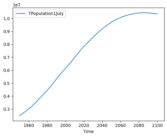
We can thus see that the world population is projected to continue growing for the next 50 years or so. But by the year 2100, growth will slow down, and maybe we’ll even start to see a decline in population. I’ve put it on my calendar for January 2100, to examine the data for Bamboo Weekly.