


[Administrative note: I'll be holding office hours for paid subscribers, including members of my Python+data membership program, on this coming Sunday, August 18th. Come with any and all Pandas questions; my goal is to answer anything I can. I'll send a reminder and Zoom link tomorrow.]
This week, we're looking at cyber attacks, which have been in the news quite a bit. The most prominent mentions have been Russian breakins into Microsoft's systems (https://edition.cnn.com/2024/03/08/tech/microsoft-russia-hack/index.html) and Iranian breaks into the Trump campaign (https://www.nytimes.com/2024/08/11/us/politics/trump-campaign-hacking-iran.html?unlocked_article_code=1.C04.wwrD.02yxkx89ZYzT&smid=url-share). Just yesterday, Politico reported that Google confirmed Iranian attempts to break into both the Biden (now Harris?) and Trump campaigns (https://www.politico.com/news/2024/08/14/google-iran-hackers-trump-biden-campaign-00174046).
Even when they aren't front-page headlines, such attacks take place all the time. And why not? They're easy and cheap to pull off, and can be hugely effective. I strongly recommend "The Perfect Weapon," the book by NY Times reporter David Sanger that opened my eyes to some of the issues on this topic.
Data and six questions
This week's data set comes from the Center for International and Security Studies at the University of Maryland (https://cissm.umd.edu/). They have a database of cyber attacks dating back to 2014. You can download it from here:
https://cissm.umd.edu/research-impact/publications/cyber-events-database-home
Click on the link "publication file" on the right side of the screen, and you'll get an Excel file containing their database.
This week, I have six tasks and questions for you. The learning goals include working with dates and times, grouping, pivot tables, plotting, and string methods.
As always, a link to download the Jupyter notebook I used to solve all six questions is at the bottom of the post.
Read the data into an Excel file. Make sure that the event_date column into a datetime dtype.
Before doing anything else, let's load Pandas:
import pandas as pdI then used read_excel to read the Excel file into a data frame:
filename = 'umspp-export-2024-07-19.xlsx'
df = pd.read_excel(filename)
Normally, it wouldn't be an issue for event_date to be treated as a datetime value, because Excel has datetime columns, and those columns are usually read into Pandas with the appropriate dtype.
However, it would seem that the Excel column wasn't tagged as a datetime. For that reason, the dtype is seen as object, meaning a Python object – which normally means a Python string.
I decided that I should tell read_excel to parse the event_date column as a datetime, passing the column name (event_date) as an argument to parse_dates. For reasons I still don't quite understand, it didn't work. I was thus forced to do it manually, applying pd.to_datetime to the column, assigning it back to the event_date column:
df['event_date'] = pd.to_datetime(df['event_date'])The resulting data frame has 13,668 rows and 16 columns, each describing a cyber security event recorded by the CISSM.
Create a line plot showing the number of incidents in each month. Has the number of incidents grown consistently over time?
In order to plot the number of incidents each month, we'll need to count them. We can do that by running groupby on both the year and the month in the event_date column. (If we were to just group on the month, then we would know how many incidents occur in January vs. February vs. March, etc., across all years.)
We can group on multiple columns by passing a list of columns to groupby. And we can retrieve the year and month from a datetime column using the dt.year and dt.month accessors. Our query will thus look like this:
(
    df
    .groupby([df['event_date'].dt.year,
              df['event_date'].dt.month])
    ['slug'].count()
)
Notice that I need to pick a column to count; in this case, I chose slug, but it really doesn't matter, so long as the column doesn't have any NaN values. The count method returns the number of non-NaN values for each combination of year and month. groupby sorts its results by default, meaning that the series we get back will be sorted chronologically, from earliest to latest year-month combinations.
To find out whether there has been an increase or decrease over time, we can then invoke pct_change, which tells us how much each month changed from the previous one. We can then sum those values, to find out the overall change from the start of the data set to the end:
(
    df
    .groupby([df['event_date'].dt.year,
              df['event_date'].dt.month])
    ['slug'].count()
    .pct_change()
    .sum()
)
I get a 95% increase, meaning that it has nearly doubled in the decade during which CISSM has been tracking security incidents.
We can plot this by using plot.line on the result of the groupby:
(
    df
    .groupby([df['event_date'].dt.year,
              df['event_date'].dt.month])
    ['slug'].count()
    .plot.line()
)
I get the following plot:
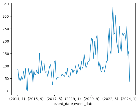
Notice that the number of incidents in 2024 appears to have plunged – but that doesn't mean we're doing well. Rather, it just reflects the fact that there were very few reports in the CISSM database so far, because it takes a while for things to be reported and then entered.
Find the 5 countries in which the greatest number of incidents have occurred. Plot the number of incidents per month, for each of these countries.
First, we need to find the five countries where the greatest number of incidents occurred. The easiest way to do that is with value_counts, applied to the country column. That'll return a series in which the country names provide the index and the number of incidents for each country provides the value:
df['country'].value_counts().head(5).index)We can then use head(5) to retrieve the five most commonly mentioned countries; this works, because value_counts automatically sorts its results from most to least common. Finally, we take the index attribute from that five-element series, to get just the country names.
We did this in order to know which countries truly interest us. Now that we have found those countries, we want to filter the data frame, keeping only those rows where the country appears in that list. For this, we can use the isin method inside of a call to loc:
(
    df
    .loc[lambda df_: df_['country'].isin(df['country']
                                         .value_counts()
                                         .head(5)
                                         .index)]
)
loc always allows to retrieve specific rows from a data frame. Here, we pass lambda, which returns a boolean series indicating where we should keep the row, and where we should reject it.
Having kept only those rows that are of interest, we can now create a pivot table:
- The rows, aka the index, will contain a combination of year and month, as we did before in our
groupby. - The columns will be for the countries.
- The values will come from
slug, which we've already used for similar purposes. - The aggregation function will be
count, checking the number of incidents.
Here's how we can create the pivot table:
(
    df
    .loc[lambda df_: df_['country'].isin(df['country']
                                         .value_counts()
                                         .head(5)
                                         .index)]
    .pivot_table(index=[df['event_date'].dt.year,
                        df['event_date'].dt.month],
                 columns='country',
                 values='slug',
                 aggfunc='count')
)
The resulting data frame contains 121 rows and five columns. We can then know, for each of the five most-common countries, the number of attacks that took place there in every month and year.
(
    df
    .loc[lambda df_: df_['country'].isin(df['country']
                                         .value_counts()
                                         .head(5)
                                         .index)]
    .pivot_table(index=[df['event_date'].dt.year,
                        df['event_date'].dt.month],
                 columns='country',
                 values='slug',
                 aggfunc='count')
   .plot.line()
)
That gives us the following plot:
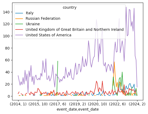
We can see that the number of cyberattacks against the United States is far greater than any other country, with the exception of June 2022, when Russia suffered a large number of attacks. I'm going to guess that this was related to their invasion of Ukraine; we can similarly see that there was a spike in attacks against Ukraine in 2023, as part of a Russian cyber-attack front.
What are the 10 most commonly cited actors (i.e., perpetrators) of cyber crime whose actor country can be determined? What types of actors are they, and where are they from? Does any one country seem to be behind most of these? Restrict actor names to only 40 characters.
If we were previously interested in the five countries on the receiving end of cyber attacks, now we're interested in who is performing these attacks, known as "actors" in the database.
First, we'll keep only three columns (actor, actor_type, and actor_country). Then we'll use loc and lambda to remove rows in which actor_country is Undetermined. That accounts for a large number of attacks, and I hate to throw out so much data... but at the same time, we can't exactly claim that Undetermined is behind a lot of cyber attacks for this analysis:
(
    df
    [['actor', 'actor_type', 'actor_country']]
    .loc[lambda df_: df_['actor_country'] != 'Undetermined']
)
If we were in a regular Python program, and wanted to truncate strings after 40 characters, we could use a slice, as in s[:40]. Note that even if a string is shorter than 40 characters, we can always apply a slice with an endpoint that goes beyond the edge – in contrast with asking for a particular index, in which case we'll get an exception.
How can we apply a slice to all of these strings? With the str.slice method, which takes either two or three arguments. These match the slice builtin in Python. Most people don't know about this builtin, because they just use the : syntax inside of square brackets, which is fine. The only tricky part is that you can simulate leaving something blank when you call slice (or str.slice) by passing None instead of a value.
We can thus get the truncated place names in this way:
(
    df
    [['actor', 'actor_type', 'actor_country']]
    .loc[lambda df_: df_['actor_country'] != 'Undetermined']
    .assign(actor = lambda df_: df_['actor'].str.slice(None, 40))
)
I then repeated this, passing a second keyword argument to assign, for the actor country, just to make things more readable:
(
    df
    [['actor', 'actor_type', 'actor_country']]
    .loc[lambda df_: df_['actor_country'] != 'Undetermined']
    .assign(actor = lambda df_: df_['actor'].str.slice(None, 40),
           actor_country = lambda df_: df_['actor_country'].str.slice(None, 40),
           )
)
Finally, we can invoke value_counts on the three-column data frame. This will return a series with a three-part multi index, one part for each of the columns in the data frame on which we can value_counts. We can then invoke head(10) to get the 10 most-common actors:
(
    df
    [['actor', 'actor_type', 'actor_country']]
    .loc[lambda df_: df_['actor_country'] != 'Undetermined']
    .assign(actor = lambda df_: df_['actor'].str.slice(None, 40),
           actor_country = lambda df_: df_['actor_country'].str.slice(None, 40),
           )
    .value_counts()
    .head(10)
)
Here are the result; I changed the truncation size to 20 characters, so that it would fit nicely into this format:
actor                 actor_type    actor_country
cl0p                  Criminal      Russian Federation      301
NoName057(16)         Hacktivist    Russian Federation      269
NGB 3rd Technical Su  Nation-State  Korea (the Democrati    148
ALPHVM                Criminal      Russian Federation      123
GRU Main Special Cen  Nation-State  Russian Federation      118
Black Basta           Criminal      Russian Federation       99
Killnet               Hacktivist    Russian Federation       96
WIZARD SPIDER         Criminal      Russian Federation       84
OurMine               Hobbyist      Saudi Arabia             73
REvil                 Criminal      Russian Federation       68
Name: count, dtype: int64
As we can see, a very large number of the bad actors here are from Russia. Some are classified as criminals, some are "hacktivisits," and some are from the state itself. But this confirms what experts have long said, namely that Russia is quite the world power when it comes to cyber attacks.
What are the 20 most common words, containing at least 5 letters, that occur in the incident descriptions? How often do they occur? Ignore leading and trailing punctuation on the words, as well as "words" that contain garbage characters.
To answer this question, we'll focus on the description column. To that end, we'll start by saying:
(
    df
    ['description']
)
If we were in a regular Python program, we would break a string into individual words using the str.split method. Fortunately, Pandas offers us an almost identical method, also known as str.split, which we apply via the str accessor:
(
    df
    ['description']
    .str.split()
)
This returns a series containing Python lists. That's already a bit unusual, but we really want to work with the individual words, not lists of words. That's where the explode method comes into play; it returns a new series in which we get one row for each element of each list. In other words, it returns a series of individual words, based on our series of lists. The index, by default, remains the same as it was in the original series, although that doesn't really interest us here:
(
    df
    ['description']
    .str.split()
    .explode()
)
We now have a series of strings. But some of those strings start or end with punctuation, which I want to remove. I can thus use the str.strip method, passing it string.punctuation, a string that comes with Python's standard library.
It's most common to call str.strip without any argument, in order to remove leading and trailing whitespace. But we can pass it a string argument, in which case str.strip will remove any and all of the characters in that string from the front and back of the string. (It won't modify anything inside.)
You can think of str.strip as a form of while loop: So long as the character at index [0] or [-1] of the string is located in string.punctuation, remove the character.
Here's how we can do that:
import string
(
    df
    ['description']
    .str.split()
    .explode()
    .str.strip(string.punctuation)
)
Next, I run dropna, to remove any NaN values that we might have accumulated along the way.
Following that, I use a regular expression and str.contains to make sure that the string contains at one or more alphanumeric characters (\w+), and that it only contains such characters from the start of the string (^) to its end ($).
I then use another loc and lambda combination to check that the word contains at least five characters. I also lowercase the word, so that we won't see abc and ABC as different:
import string
(
    df
    ['description']
    .str.split()
    .explode()
    .str.strip(string.punctuation)
    .dropna()
    .loc[lambda s_: s_.str.contains(r'^\w+$', regex=True)]
    .loc[lambda s_: s_.str.len() >= 5]
    .str.lower()
)
Finally, I again run value_counts and head, and end up with the 20 most common words:
import string
(
    df
    ['description']
    .str.split()
    .explode()
    .str.strip(string.punctuation)
    .dropna()
    .loc[lambda s_: s_.str.contains(r'^\w+$', regex=True)]
    .loc[lambda s_: s_.str.len() >= 5]
    .str.lower()
    .value_counts()
    .head(20)
)
Here's what I got:
description
attack         3850
ransomware     2932
breach         2167
information    1961
after          1797
group          1345
their          1261
website        1224
company        1191
hackers        1185
claims         1059
access         1052
personal       1003
network         945
threat          944
security        919
against         919
compromised     915
email           913
hacked          880
Name: count, dtype: int64
I must say, I'm not at all surprised by what I see here.
What are the 15 top combinations of attackers and defenders from cyberattacks? Are there any instances where a country is both the attacker and defender?
To perform this analysis, we'll have to look at the country and actor_country columns. But first, let's use loc and lambda to remove any row in which the country is Undetermined:
(
    df
    .loc[lambda df_: df_['actor_country'] != 'Undetermined']
)
With that in place, we can use groupby to group by both columns. We'll use count as the aggregation function, and use slog as the column we're counting:
(
    df
    .loc[lambda df_: df_['actor_country'] != 'Undetermined']
    .groupby(['country', 'actor_country'])['slug'].count()
)
This tells us how often each combination of actor_country and country are found together. However, if I want to find the top 15 values, I'll use sort_values to get them in order, and then head to get just the top 15:
(
    df
    .loc[lambda df_: df_['actor_country'] != 'Undetermined']
    .groupby(['country', 'actor_country'])['slug'].count()
    .sort_values(ascending=False)
    .head(15)
)
Since the country names were running long, I again used assign and str.slice to truncate them to 20 characters:
(
    df
    .loc[lambda df_: df_['actor_country'] != 'Undetermined']
    .assign(country = lambda df_: df_['country'].str.slice(None, 20),
           actor_country = lambda df_: df_['actor_country'].str.slice(None, 20),
           )
    .groupby(['country', 'actor_country'])['slug'].count()
    .sort_values(ascending=False)

    .head(15)
)
Here's the result that I got:
country               actor_country
United States of Ame  Russian Federation      672
Ukraine               Russian Federation      264
Russian Federation    Ukraine                  92
Poland                Russian Federation       92
United States of Ame  United States of Ame     91
United Kingdom of Gr  Russian Federation       73
United States of Ame  Saudi Arabia             67
Italy                 Russian Federation       66
Germany               Russian Federation       66
Lithuania             Russian Federation       51
India                 India                    49
Canada                Russian Federation       47
France                Russian Federation       46
Armenia               Azerbaijan               46
Italy                 Italy                    44
Name: slug, dtype: int64
First, we can see (again) that Russia is initiating a lot of attacks – especially on the United States! Numbers 2 and 3 are Russia attacking Ukraine, and Ukraine attacking Russia, which makes sense given the Russian invasion that occurred more than two years ago.
But we also see that countries are sometimes attacking themselves! This doesn't mean state actors are attacking the state (which would be weird), but that there are cases of US-based groups attacking in the US. This is also true for India and Italy.
That's it for this week's analysis. Here's a link to my Jupyter notebook: https://drive.google.com/file/d/1n0C9sZkJAs74sOZ3_NfUoykv9B4x4PSC/view?usp=sharing
I'll be back next week with my Pandas puzzles based on current events!
Reuven