This week, we looked at data from the American Centers for Disease Control (CDC) about measles outbreaks and vaccinations. This topic has been in the news lately, thanks to a large number of measles cases in Texas – primarily, it would seem, among people who were unvaccinated.

This is happening at the same time as the Trump administration is defunding and silencing large parts of the federal government, including the CDC. And at the same time, Robert F. Kennedy, Jr., the current secretary for health and human services, is a long-time opponent of vaccines.

While the CDC has slowed or stopped some of its reporting on diseases, information about measles is still available. We explored that data this week.

Data and six questions

The main page for measles-related data at the CDC is https://www.cdc.gov/measles/data-research/ . That's where you can see an up-to-date indication of how many people have been infected, how many of them were unvaccinated, and how many people died from the disease.

From that page, you can also download a number of data sets in CSV format, just after each of the relevant charts, maps, and graphs.

This week, I gave you six tasks and questions.

If you're a paid subscriber, then you'll be able to download the data directly from a link at the bottom of this post, download my Jupyter notebook, and click on a single link that loads the notebook and the data into Google Colab, so you can get to work experimenting right away.

Here are my six tasks and questions:

Read the "weekly cases by onset date" into a data frame. Create a line plot comparing the week_start column with the number of cases. Would the recent outbreak in the US seem to fit the usual pattern, or is this an unusually high number of cases?

First, let's load up Pandas. And while we're at it, we can load os, too:

import pandas as pd
import os

Why os? That module includes os.path.join, which combines strings to create a single pathname we can feed to pd.read_csv. I normally don't use os.path.join in solving these problems, but there were multiple data files, and I decided to put them all into a single subdirectory (data/bw-108). This just made it easier.

The first thing I did was thus run read_csv on the result of invoking os.path.join, combining the directory name with the CSV file's name:

df = pd.read_csv(os.path.join(dirname, 'weekly-cases-by-onset-date.csv')
)

But while loading the CSV file, I wanted to change things a bit. First, I only needed to load two columns, week_start and cases. I thus passed the usecols keyword argument, naming the two columns I wanted to keep from the file. This not only helps to make our data frame more manageable and readable, but reduces the amount of memory the data frame consumes:

df = pd.read_csv(os.path.join(dirname, 'weekly-cases-by-onset-date.csv'),
               usecols=['week_start', 'cases']
)

But I also wanted to treat the week_start column in two special ways: First, I told Pandas to treat it as a datetime type, as opposed to a string. We can do that with parse_dates, which works just fine on unambiguously formatted dates, like we have here.

I also wanted to use the week_start column into the data frame's index. I did that by passing the index_col keyword argument:

df = pd.read_csv(os.path.join(dirname, 'weekly-cases-by-onset-date.csv'),
               usecols=['week_start', 'cases'],
                parse_dates=['week_start'],
                 index_col='week_start')

The result of this command is a data frame with 113 rows and 1 column containing cases. This is not quite the same as a series, although it's very close to one.

I then asked you to plot the number of cases during each week for which we have data. Fortunately, we can use the Pandas interface to Matplotlib, which I find far easier to use. We just invoke plot.line on the data frame:

df.plot.line()

That produces the following plot:

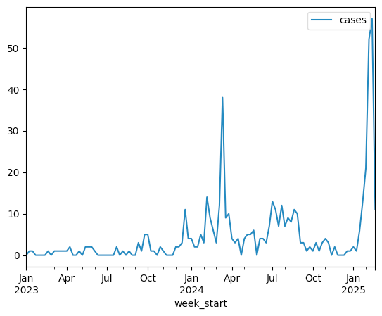
From this plot, we can see that the US is currently encountering a far larger spike in measles cases than at any point during the last two years. And the numbers are presumably only growing, at least for now.

The CDC says that measles isn't a seasonal disease. Let's try to see that visually, using data from 2023 and 2024: Create a new line plot, whose x axis represents the months of the year. Plot the number of cases from each 2023 and 2024 using a separate line, in a different color. Do we see any obvious common peaks or dips between the two years?

When we plot a single-column data frame or a series, we get (as we saw above) a single line. If we plot a two-column data frame, then we get two lines, both against the same x and y axes.

What we want, then, is to take our existing data frame and then restructure it such that the index contains the names of the months, the columns contain the years (2023 and 2024), and the values represent the total number of cases in each month. How can we do that?

First, I took advantage of the fact that when we have datetime values in our index, and when the values are sorted, we can use loc and a slice to retrieve a limited set of rows. If we give only part of a date, then the smaller-sized parts of the datetime all match. I thus looked for ['2023':'2024'], which gave me all rows from 2023 and 2024. Note that while Python slices are normally "up to and not including," loc always returns values up to and including:

(
    df
    .loc['2023':'2024']
)

Next, I decided to create two new columns, month and year, with the month and year of each entry. I can do that with assign, which creates a (temporary) new column with the name and value that we assign. It's typical to pass a lambda expression as the value, providing a function that Pandas invokes to get the values in real time.

But to do that, I first have to run reset_index, so that we can address the column as an actual column, rather than the index:

(
    df
    .loc['2023':'2024']
    .reset_index()
    .assign(month = lambda df_: df_['week_start'].dt.month_name(),
            year = lambda df_: df_['week_start'].dt.year)
)

While this worked, it also gave me a bad feeling. Surely there's a more elegant way to do this, right?

Then I remembered that our index contains datetime values: We can access it directly via df.index, and then invoke any of the datetime-related methods and attributes we want.

It's tempting to thus say:

(
    df
    .loc['2023':'2024']
    .assign(month = df.index.month_name(),
            year = df.index.year)
)

However, this will result in an error. That's because the call to loc in the second line returns a new data frame, one with a smaller (and different) index than the original df. Which means that if we then try to use assign and values from df.index, there will be a mismatch.

We thus need to reorder things, first running assign and only then filtering by year with a slice:

(
    df
    .assign(month = df.index.month_name(),
            year = df.index.year)
    .loc['2023':'2024']
)

Notice two things here: First, when we retrieve datetime attributes from the index, we don't need to use the dt accessor. Second, month_name is a method, whereas year is data. So the first needs (), but the second cannot take them. If you find this inconsistent and confusing... well, you're not alone!

With this in place, we can now invoke pivot_table to get our pivot table back, using the months as rows, the years as columns, the values from cases, and then the aggregation function sum to add up all of the values in each month-year cell:

(
    df
    .assign(month = df.index.month_name(),
            year = df.index.year)
    .loc['2023':'2024']
    .pivot_table(index='month',
                 columns='year',
                 values='cases',
                 aggfunc='sum')
)

Finally, we can invoke plot.line to plot these two lines against each other:

(
    df
    .assign(month = df.index.month_name(),
            year = df.index.year)
    .loc['2023':'2024']
    .pivot_table(index='month',
                 columns='year',
                 values='cases',
                 aggfunc='sum')
    .plot.line()
)

Here's what we get:

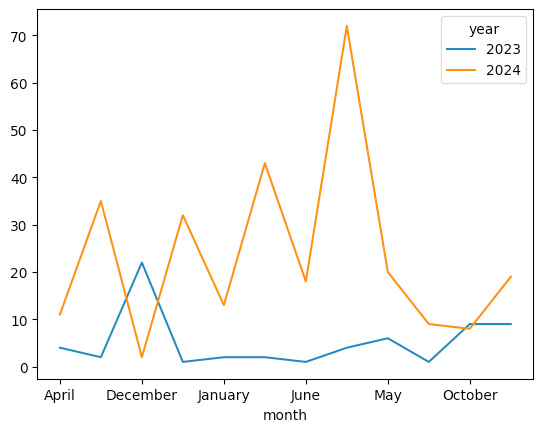
Does this graph look a bit funny to you? Look at the x axis, where the months are... in alphabetical order. That's a lovely idea, but not very useful if we're looking at months of the year.

Grouping in Pandas always sorts the results by default, whether in a groupby or in pivot_table. If we want to turn sorting off, and get the index in its original order, we have to pass sort=False:

(
    df
    .assign(month = df.index.month_name(),
            year = df.index.year)
    .loc['2023':'2024']
    .pivot_table(index='month',
                 columns='year',
                 values='cases',
                 aggfunc='sum',
                sort=False)
    .plot.line()
)

Here's the final plot:

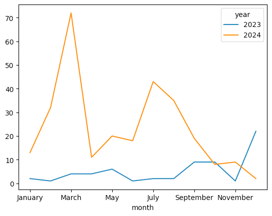
I don't see any correlation between seasons and the number of cases. There were spikes in February-March and July of 2024, but the spike in 2023 happened in December. This graph would seem to confirm the non-seasonality of measles.