


It's 2026 — can you believe it? Happy New Year to everyone. I hope that the new year gives you and those close to you health, happiness, and peace. I'm grateful that you spend some time with me each week here at Bamboo Weekly (and with my other Python-related learning materials).
This week's topic is PyPI (https://pypi.org), the online repository for Python packages that's essential to the Python ecosystem. PyPI is managed by the Python Software Foundation; if you haven't joined to support the development of Python, you can still do so at https://www.python.org/psf/membership/. You'll even get to vote in the annual board elections, giving you a voice on the future direction of the Python language and community.
Data and five questions
PyPI is so huge, and so popular, that download statistics aren't available directly. Rather, you have to get them from a project at Google's BigQuery. I had thought several times about using BigQuery, but shied away from it because it seemed big, daunting, and complex.
There is a PyPI project called pypinfo (https://pypi.org/project/pypinfo/) that seems to provide an easy-to-use Python API for BigQuery, allowing you to construct queries and get Pandas data frames back. But despite the documentation's claims that signing up for a BigQuery user, project, and key shouldn't be hard, I managed to mess it up several times.
I finally turned to Claude, which both walked me through the process and then convinced me that I should just use BigQuery's SQL syntax directly. I ended up with a number of Python programs that I shared with you, each of which performs a query against BigQuery, produces a Pandas data frame as a result, and then exports that data frame to a file in "parquet" format.
If you struggled with getting these programs to work, then you're not alone! Paid subscribers can avoid some of the pain (but also some of the learning) and get the data files from the end of this message. If things don't work for you, then I would suggest using Claude, ChatGPT, or whatever GenAI chatbot you prefer, and use it to look at the code, look at the error messages you're getting, and also the screenshots you're seeing on the Google Cloud console. I find that sharing error messages and screenshots goes a long way toward debugging with AI.
Here are the programs:
Note that each of the programs, as written, assumes:
- You have defined a project called
bw-151in BigQuery. You can call a project whatever you want, and it could be the same as mine or different. - BigQuery gives you access using keys, with each key associated with one user. I downloaded the key in JSON format, and then put it in a file on my computer. However, the program expects to find the key in an environment variable called
GOOGLE_APPLICATION_CREDENTIALS. I could have just set it on the command line, but decided to use theosmodule to setos.environ, which has the effect of changing the environment for the current process. You can choose between saving the downloaded key into a file, and then just changing the path to that file from my program, or perhaps setting the environment variable in your startup shell.
Some of these programs took a few minutes to run, but none of them took a very long time, in part because I made sure to limit their scope. I assumed that by saving them in parquet format, I wouldn't have issues loading the data; parquet is part of the Apache Arrow project, and is meant to be a small, portable binary format that can be used by Pandas and many other programs.
And that happens to be true! But it's also true that (unbeknownst to me when I started) the dates in the parquet files were all a special Google version of dates, rather than the standard datetime64 that we know and love. One solution would have been to open each file, run pd.to_datetime on each date value, and then re-save the file. I found, however, that by using a PyArrow backend for the data frame, things worked just fine. And while PyArrow-backed data frames aren't yet considered stable or production ready, we should be fine for this small set of data.
Paid subscribers to Bamboo Weekly, or to my LernerPython membership program (at https://LernerPython.com), can download the data files from the end of this message, as well as my Marimo notebooks. They also get one-click access to my notebook at Molab, the Marimo space for sharing notebooks. Paid subscribers also get access to all BW questions and answers and an invitation to monthly office hours.
Learning goals for this week include: Loading Parquet files, dates and times, pivot tables, and plotting.
Here are my five questions and tasks for this week:
Read the "daily downloads" data into a Pandas data frame. (The Parquet files was written using a weird type that Arrow and PyArrow can handle, but pure Pandas cannot. So use dtype_backend='pyarrow', in order for it to work.) Was the mean number of downloads higher on weekends or weekdays? PyCon US took place from May 14-18, 2025. Was the mean on those days higher or lower than the rest of the year? (And by how much did it differ?) On which 5 days were there the most downloads? The fewest?
I ran the "daily downloads" program, which looked like this:
#!/usr/bin/env uv run python3

from google.cloud import bigquery
import pandas as pd
import os

print('Starting...')

# Set your project
os.environ['GOOGLE_APPLICATION_CREDENTIALS'] = '/Users/reuven/Downloads/bw-151-0ffffc35f2a0.json'

# Create client with explicit project
client = bigquery.Client(project='bw-151')

query = """
SELECT
    DATE(timestamp) as download_date,
    COUNT(*) as total_downloads
FROM
    `bigquery-public-data.pypi.file_downloads`
WHERE
    DATE(timestamp) BETWEEN '2025-01-01' AND '2025-12-31'
GROUP BY
    download_date
ORDER BY
    download_date
"""

# Run query and get results as pandas DataFrame
df = client.query(query).to_dataframe()

print(f'Downloaded {len(df.index)} records. Saving to parquet...')
df.to_parquet('bw-151-daily-downloads.parquet')
print('Done.')
Notice that the first line isn't the usual #!/usr/bin/env python3 shebang line, but rather one that calls uv run python3. That ensures we're running under the current version of Python as defined by the current uv project.
I then set the environment variable with my Google API key, as well as the Google BigQuery project.
I then used a triple-quoted string to define an SQL query:
- I asked for the timestamp of each download and the number of total downloads
- I retrieved from
bigquery-public-data.pypi.file_downloads, the repository in BigQuery that contains the data - I restricted the dates to just 2025. Without doing this, the query would have taken much longer and also used more memory. And while 1TB sounds like a lot of RAM, it will quickly evaporate if you perform massive queries over long periods of time.
- I used
GROUP BY, which is (perhaps obviously) likegroupbyin Pandas, indicating that I wanted a new row of output for each distinct date - Finally, I used
ORDER BYto sort the results in chronological order.
The BigQuery response object has a to_dataframe method, which I invoked here to output a Pandas data frame. I assigned that to df, and then invoked to_parquet to save it to a file.
So far, so good! Now I just needed to write a Pandas program to open the file and start performing our queries.My first goal was to find out whether there are more downloads on weekends or weekdays.
I started by loading a bunch of modules I would need and use:
import marimo as mo
import pandas as pd
from plotly import express as px

import os
data_directory = '/Users/reuven/BambooWeekly/notebooks/data/'
In addition to importing os, I also defined data_directory. That allowed me to use os.path.join to get the full pathname for data files. Indeed, I defined the filename for daily downloads:
daily_downloads_filename = os.path.join(data_directory, 'bw-151-daily-downloads.parquet')
I used read_parquet to read the file into Pandas. But I got a weird error, one that I hadn't ever seen before:
(
    pd
    .read_parquet(daily_downloads_filename)
)
I got:
TypeError

    data type 'dbdate' not understood
    See the console area for a traceback.
I had always thought that parquet was a completely neutral format, one that could be used to store and retrieve data on any platform. And that's mostly true! But it turns out that you can store custom data structures in a parquet file, and that's what happened when I used to_dataframe from BigQuery.
Fortunately, I was able to get around this (as I mentioned above) by using the experimental PyArrow backend storage for Pandas. I'm not quite sure what it does differently, although it's likely that because both PyArrow and parquet are part of the Apache Arrow project (https://arrow.apache.org/), that it worked. Regardless, I got a data frame with:
(
    pd
    .read_parquet(daily_downloads_filename, dtype_backend='pyarrow')
)
The data frame contained two columns, download_date and total_downloads. The former was a datetime value, which means that I could use dt.dayofweek to get the day of week. And indeed, many people would check if dt.dayofweek > 4 to find out if a particular date is on the weekend.
I decided that the data frame is small enough, that I can just use dt.day_name(), a method that returns the actual day names. Paired with isin, I was able to use assign to create a new column, is_weekend, with a boolean value – True on Saturdays and Sundays, and False otherwise.
I was then able to use groupby, getting the mean number of downloads on weekends and non-weekends:
(
    pd
    .read_parquet(daily_downloads_filename, dtype_backend='pyarrow')
    .assign(is_weekend = lambda df_: df_['download_date'].dt.day_name().isin(['Saturday', 'Sunday']))
    .groupby('is_weekend')['total_downloads'].mean()
)
The result:
is_weekend	total_downloads
false	2764869718.3256707
true	1719638873.2403846
In other words, there is an average of 1.7 billion downloads from PyPI, per day, on weekends. But that number rises to about 2.8 billion downloads per day from PyPI during the week.
I was similarly curious to know if PyPI downloads change during PyCon US. On the one hand, you might expect them to rise, because there's lots of intense Python activity going on, and everyone is motivated to do a lot. On the other hand, you might argue that conference attendees are all attending talks, and thus aren't running uv add every 10 seconds. (Although let's be honest: Lots of people attending conference talks are also on their laptops, often coding...)
Here, I used similar code to what we saw before. But the lambda expression I used in this call to assign, setting the boolean column is_pycon_us, used pd.date_range, a method that you don't often use... until it really comes in handy. After creating that boolean column, I again used groupby:
(
    pd
    .read_parquet(daily_downloads_filename, dtype_backend='pyarrow')
    .assign(is_pycon_us = lambda df_: df_['download_date'].isin(pd.date_range('2025-05-14', '2025-05-18')))
    .groupby('is_pycon_us')['total_downloads'].mean()
)
The results:
is_pycon_us	total_downloads
false	2470885798.072222
true	2190910398.8
We actually do see a drop in PyPI downloads during PyCon US, from about 2.5 billion requests/day to 2.2 billion. However: You could argue that the drop is due, in part, to the fact that PyCon US takes place over a weekend, which (as we saw) has a much lower rate of downloads.
Finally, I wanted to know when PyPI downloads are the highest and lowest. I did that by invoking set_index on the data frame, turning the download date into the index, and then invoking nlargest and nsmallest together (via agg). I then used sort_index so that we could see the dates in chronological order. I also used [] to retrieve the total_downloads column, to avoid a multi-index in the output:
(
    pd
    .read_parquet(daily_downloads_filename, dtype_backend='pyarrow')
    .set_index('download_date')
    .agg(['nlargest', 'nsmallest'])
    .sort_index()
    ['total_downloads']
)
The result:
download_date	nlargest	nsmallest
2025-01-01T00:00:00.000		1170377988
2025-01-04T00:00:00.000		1128371223
2025-01-05T00:00:00.000		1105777472
2025-01-12T00:00:00.000		1152397247
2025-01-19T00:00:00.000		1149310785
2025-11-19T00:00:00.000	3889005787
2025-12-02T00:00:00.000	3941696642
2025-12-03T00:00:00.000	4021548951
2025-12-04T00:00:00.000	3896483024
2025-12-09T00:00:00.000	3878840019
In other words, we saw very low download rates at the start of the year, in January. The largest rates were in mid-November and the start of December. I cannot think of a specific reason why these dates would be so high or low, other than (for example) the very small number of people working on New Year's Day. (Um, that includes me, but whatever...)
The uv package manager has become extremely popular over the last year. (I've even created a free 15-part e-mail course, which you can take at https://uvCrashCourse.com.) I'm curious to know if uv has improved its market share over the course of the year. Read the per-day, per-installer data into a Pandas data frame. Create a stacked bar plot showing the proportion of downloads used by each installer. Do you see an obvious increase in the use of uv? Is there a percentage increase in uv over time?
I once again used os.path.join to define the filename I wanted to load and use. (I'm not going to review the file itself, or the BigQuery program used to retrieve it, because it's similar to what we saw before.) I again used read_parquet, specifying a dtype_backend of pyarrow:
installer_downloads_filename = os.path.join(data_directory, 'bw-151-installer-per-day.parquet')
(
pd
.read_parquet(installer_downloads_filename, dtype_backend='pyarrow')
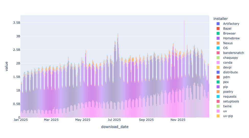
)I wanted to create a stacked bar plot for each of the installers, but doing that on a per-day basis for the entire year would create a hard-to-read plot:
I thus decided to do it on a month-t0-month basis. I used assign and dt.month to get the month from each stat. I then used pivot_table to create a new data frame in which the months were the rows and the different installers were the columns:
(
    pd
    .read_parquet(installer_downloads_filename, dtype_backend='pyarrow')
    .assign(month = lambda df_: df_['download_date'].dt.month)
    .pivot_table(index='month',
                columns='installer',
                values='downloads',
                aggfunc='sum')
)
With this pivot table in place, I used pipe, which lets us invoke a function as if it were a method on data frames, passing it px.bar, creating a bar plot. Better yet, by default px.bar creates a stacked bar plot, using each column as a different color:
(
    pd
    .read_parquet(installer_downloads_filename, dtype_backend='pyarrow')
    .assign(month = lambda df_: df_['download_date'].dt.month)
    .pivot_table(index='month',
                columns='installer',
                values='downloads',
                aggfunc='sum')
    .pipe(px.bar)
)
The result:
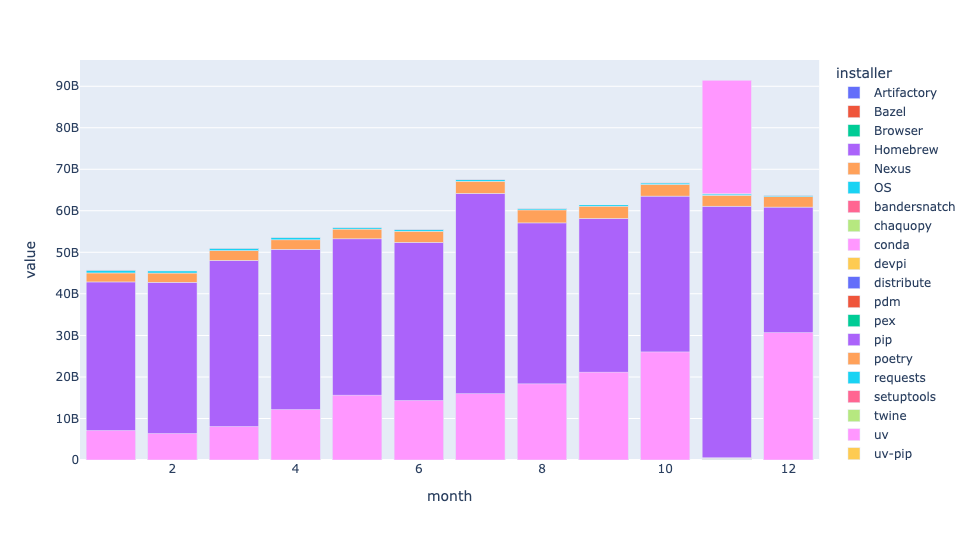
First: I had no idea that there were so many different installers in the Python world! I figured that there was pip (obviously), uv, conda, and maybe a handful of others. But OMG, there were so many.
Each bar represents total downloads for that month. You can see a slow-but-steady increase in how many packages are downloaded each month, demonstrating that Python continues to grow in popularity.
The dark purple part of each bar is pip, and it makes sense that it's the largest part of each bar. But uv, in the pink, is clearly growing, as well. With each passing month, you can see more and more of each bar in pink, showing the dramatic growth of uv in just the last year.
By the way, why is the uv bar on top for November, rather than on the bottom, as it is every other month? I dunno!
What is the increase in uv use over time? I started with the same query as I used above, with one change to my call to pivot_table, namely the margins=True keyword argument. Because my aggregation function was sum, this gave me the total number of downloads for each month (at the end of each row) and the total number of downloads for each tool (at the end of each column):
(
    pd
    .read_parquet(installer_downloads_filename, dtype_backend='pyarrow')
    .assign(month = lambda df_: df_['download_date'].dt.month)
    .pivot_table(index='month',
                columns='installer',
                values='downloads',
                aggfunc='sum',
                 margins=True)
)
I then used assign to create a new column, uv_percentage, dividing the values in the uv column into the values in the All column. That gave me the percentage of total downloads executed by uv. I grabbed that column with [], and then invoked px.bar via pipe:
(
    pd
    .read_parquet(installer_downloads_filename, dtype_backend='pyarrow')
    .assign(month = lambda df_: df_['download_date'].dt.month)
    .pivot_table(index='month',
                columns='installer',
                values='downloads',
                aggfunc='sum',
                 margins=True)
    .assign(uv_percentage = lambda df_: df_['uv']/ df_['All'])
    ['uv_percentage']
    .pipe(px.bar)
)
The result:
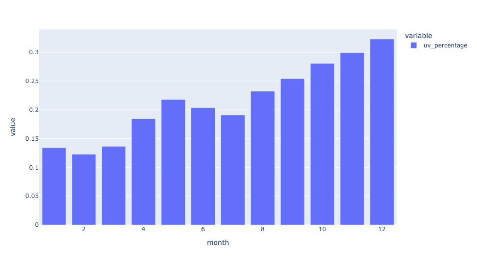
We can see that in January, uv was less than 15 percent of downloads from PyPI. By the end of the year, it was more than 30 percent of all downloads.
In a word: Wow.