BW #4: Eating well (solution)

This week’s topic: Vegetables

This week, we’re looking at data from the CDC’s NSCH, focusing on children who rarely eat any vegetables. I asked you to:

1. Download the topical data file, in SAS format, from:

   https://www2.census.gov/programs-surveys/nsch/datasets/2021/nsch_2021_topical_SAS.zip. Turn it into a data frame. We're only interested in the following columns:

   • FIPSST

   • VEGETABLE

   • FRUIT

   • SUGARDRINK

2. Turn the FIPSST column into an integer, and make it the index.

3. What percentage of children had, on average, less than one vegetable per day during the week preceding the study?

4. What percentage of children had, on average, less than one vegetable per day and less than one fruit per day during the week preceding the study?

5. What percentage of children had, on average, less than one vegetable per day and less than one fruit per day and did have a sugary drink during the week preceding the study?

6. Download the FIPS state reference info, in CSV format, from https://www2.census.gov/geo/docs/reference/state.txt. Turn this into a data frame, with the STATE column as the index. The only other column we care about is STATE_NAME.

7. What percentage of children, per state, had, on average, less than one vegetaable per day during the week preceding the study?

There’s a lot to deal with here, so let’s get to it!

Discussion

The first thing that I asked you to do was import a data file stored in SAS format. Now, I’ve never used SAS, and I don’t know much about its data files. But it turns out that not everyone distributes their data in CSV or Excel files; if your organization uses SAS, then why not store things in SAS’s format? I’m sure (again, speaking from ignorance) that there are some advantages to it, such as binary storage and not having to infer dtypes.

What happens when a Pandas user encounters a SAS file? My initial guess was that I’d have to convert it to CSV. But it turns out that Pandas has a read_sas function that allows you to create a data frame directly from a SAS file.

There were two different issues that we had to deal with in opening the file. First, the data file came inside of a zipfile, so we couldn’t open it directly via a URL. We had to open the zipfile up, and then run read_sas on the file in SAS 7 format, which is what Pandas supports. That’s the file with a “sas7bdat” extension, weighing in at 182 MB.

The second problem with read_sas is that it doesn’t let you choose which columns you want in your data frame with a “usecols” keyword argument. I was thus forced to read the entire file into a data frame, and then pare that data frame down by stating which columns I wanted:

filename = '/Users/reuven/Downloads/nsch_2021_topical_SAS/nsch_2021_topical.sas7bdat'

df = pd.read_sas(filename)
df = df[['FIPSST', 'VEGETABLES', 'FRUIT', 'SUGARDRINK']]

This all seems fine, until we look at our data frame:

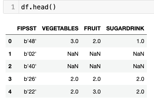
See how the FIPSST column’s values look? That seems kind of weird, no? And indeed, that column must have been stored in SAS as bytes, which were then read into Pandas as bytes, or one-character byte strings. We want integers, though, not bytes. And this means running the FIPSST column, which indicates which US state or territory is being referenced, through “astype”:

df['FIPSST'] = df['FIPSST'].astype(np.int8)

Since there are only a few dozen values for FIPSST, I decided that I’d use np.int8 for the dtype. I thus invoked “astype(np.int8)” on my column, getting back a new series, which I then assigned back to df[‘FIPSST’].

With this in place, the dtypes are all set correctly. We can thus finish up the first question by making the FIPSST column our data frame’s index (calling set_index):

df = df.set_index('FIPSST')

We’re now set to start answering some of the questions that I had posed.

I started by asking: What percentage of children had, on average, less than one vegetable per day during the week preceding the study?

In order to know this, we’ll have to learn something about the data set we’re viewing. To some degree, we can do this by reading through the data dictionary, or as they call it, the “codebook.” This is a great little Web application that can explain any of the columns in the study. If you didn’t find it yourself, the codebook is here: https://www.census.gov/data-tools/demo/uccb/nschdict.

In addition to FIPSST, which is just a numeric identifier for a state or territory, there are also three data columns:

1. VEGETABLES, a categorical column describing how many vegetables the child ate in the last week:

   1. 1 = This child did not eat vegetables

   2. 2 = 1-3 times during the past week

   3. 3 = 4-6 times during the past week

   4. 4 = 1 time per day

   5. 5 = 2 times per day

   6. 6 = 3 or more times per day

2. FRUIT, like to VEGETABLES, is a categorical column describing how many pieces of fruit the child ate in the last week:

   1. 1 = This child did not eat fruit

   2. 2 = 1-3 times during the past week

   3. 3 = 4-6 times during the past week

   4. 4 = 1 time per day

   5. 5 = 2 times per day

   6. 6 = 3 or more times per day

3. SUGARDRINK, which describes how many sugary drinks the child had in the last week:

   1. 1 = This child did not drink sugary drinks

   2. 2 = 1-3 times during the past week

   3. 3 = 4-6 times during the past week

   4. 4 = 1 time per day

   5. 5 = 2 times per day

   6. 6 = 3 or more times per day

If I want to find the children who had, on average, less than one vegetable per day, then that’ll match values 1, 2, and 3 for the VEGETABLES column. I can set up the query:

df['VEGETABLES'] < 4, 'VEGETABLES'

Remember that when we’re comparing the value < 4, we’re not saying “fewer than 4 vegetables,” but rather that the category is 1, 2, or 3. Because we’re using a boolean operator (<), we get back a boolean series. We can use that boolean series as a mask index on df, getting only those rows representing households where the children ate, on average, less than one vegetable per day:

df.loc[df['VEGETABLES'] < 4, 'VEGETABLES']

As always when we use .loc, the first argument is our row selector, and our second argument is our column selector. We’re thus asking for the VEGETABLES column in df, but only where the value of VEGETABLES is less than 4.

We don’t really want the values themselves. Rather, we want to know how many such people fit this description. We can do that with the “count” method:

df.loc[df['VEGETABLES'] < 4, 'VEGETABLES'].count()

Now we know how many people fit this description. But in order to really understand it, we’ll need it as a percentage of the entire population. To do that, we can count the number of rows in the VEGETABLES column, and then divide our previous result by it:

df.loc[df['VEGETABLES'] < 4, 'VEGETABLES'].count() / df['VEGETABLES'].count()

I get a result of 0.47. Meaning that 47 percent — just less than half! — of children 5 and under in the United States are eating less than one vegetable per day. Wow.

Next, I asked what percentage of children had, on average, less than one vegetable per day and less than one fruit per day during the week preceding the study? Maybe the children didn’t have any vegetables, but everyone likes fruit, right?

Let’s once again start with the comparison, our boolean operator. The FRUIT column uses the same values as the VEGETABLES column. We thus want to find responses where the value of VEGETABLES < 4, and the value of FRUIT is also < 4.

What we’ll do is perform each of these queries separately, getting back two separate boolean series. We’ll then run a logical “and” on these two series, getting back a new boolean series — one whose values will only be True where the input series were both True. We have to use & here, rather than “and”, because we’re not using a boolean operator. And we have to use parentheses around the two comparisons, to avoid operator precedence problems:

(df['VEGETABLES'] < 4) & (df['FRUIT'] < 4)

That gives us back a boolean series. We can apply it as a mask index to df.loc:

df.loc[(df['VEGETABLES'] < 4) & (df['FRUIT'] < 4)]

Once again, we only need the VEGETABLES column, in order to count the rows that emerged. We’ll thus use .loc with its second argument, the column selector:

df.loc[(df['VEGETABLES'] < 4) & (df['FRUIT'] < 4), 
       'VEGETABLES']

Let’s count the number of rows that result from this query:

df.loc[(df['VEGETABLES'] < 4) & (df['FRUIT'] < 4), 
       'VEGETABLES'].count()

Finally, let’s get the percentage of respondents fitting this bill by dividing the result into the total number of rows in the VEGETABLES column:

df.loc[(df['VEGETABLES'] < 4) & (df['FRUIT'] < 4), 
       'VEGETABLES'].count() / df['VEGETABLES'].count()

I got about 0.26, which means that about one quarter of young children in the US eat less than one fruit or vegetable each day.

Let’s get even more depressed, asking a more complex question: What percentage of children had, on average, less than one vegetable per day and less than one fruit per day and did have a sugary drink during the week preceding the study?

This query will be almost exactly the same as the ones above, except that it’ll also add a check for the SUGARDRINK column being greater than 1:

df.loc[(df['VEGETABLES'] < 4) & 
       (df['FRUIT'] < 4) &
       (df['SUGARDRINK'] > 1), 
       'VEGETABLES'].count() / df['VEGETABLES'].count()

Notice that I take advantage here of the fact that when you open parentheses in Python, you can largely ignore indentation issues. I find that this makes the queries easier to read.

I get a result of 0.159, or about 16 percent. Meaning that 16 percent of young US children aren’t having fruits or vegetables, but are having sugary drinks.

But of course, this describes the US as a whole. Maybe things aren’t the same across different states? The data frame already has a unique code for each state, which we’re currently using as an index. We could use a “groupby” on those codes, and find out which states are doing better, and which are doing worse.

That sounds great, except that we’ll then see the state codes, rather than the names themselves. How can we get results that’ll include state names?

Fortunately, we can download a separate data frame, one in which the index contains the same numeric codes, and whose values are the state names. Then we can join the two data frames together, getting results that are more understandable and useful.

For starters, let’s download the data from the US Census site with read_csv:

fips_url = 'https://www2.census.gov/geo/docs/reference/state.txt'

fips_df = pd.read_csv(fips_url, 
                      sep='|',
                      usecols=['STATE', 'STATE_NAME'],
                     index_col='STATE')

The above code creates a data frame from a CSV file that’s available online. But the CSV file uses vertical bars to separate fields, and it has more columns than we really need. I’ll only grab the STATE and STATE_NAME columns, and then I’ll set STATE to be the index of the resulting data frame.

With that in hand, I run a “join” on the two data frames.

joined_df = df.join(fips_df)

Now, join can be a complex beast. But in this case, it’s doing something that I hope is fairly straightforward: It returns a new data frame in which each row contains data from one row in df, and another row in fips_df. How does it know how to match the rows? Using the index.

The first row of df (i.e., df.loc[0]) has an index value of 48. When joined with fips_df, Pandas will find the row whose index is 48 (for Texas). The resulting row will have four columns: VEGETABLES, FRUIT, and SUGARDRINK from df, and STATE_NAME from fips_df. I decided to assign the result of the join to a variable, for easier manipulation:

joined_df = df.join(fips_df)