


Consumer finances
This week, we explored a small part of the data that the Federal Reserve used in its Survey of Consumer Finances, a study of that they conduct every three years about American households’ financial state.

The latest edition of the SCF was just released last week, with the report downloadable from /content/files/publications/files/scf23.pdf. Given that the report has nine (!) co-authors, it’s no surprise that there is a ton of data to review and analyze, and many questions that we could answer.
Data and seven questions
This is a weekly newsletter about Pandas, rather than a year-long, graduate-level seminar in economics — so I asked you to look at one Excel file that summarizes the data found in the research report. That file still contains many tabs, many of which describe a great deal of data, so we’re really looking at the tiniest tip of the iceberg here.
The Excel file we’re looking at is located at /content/files/econres/files/scf2022_tables_public_nominal_historical.xlsx. If you’re generally interested in the SCF, you can find out more at https://www.federalreserve.gov/econres/scfindex.htm.
This week, I gave you seven questions and tasks. The learning goals include working with Excel files (including rejiggering spreadsheets into useful data frames), multi-indexes, and plotting. A link to the Jupyter notebook that I used in solving these problems is below. Meanwhile, let’s look at how I solved things:
Create a data frame from the first two sheets (Table 1, 89-98 and Table 1, 01-22), where the index will be the descriptions (in column A) of rows 34-37, and the values will come from each year's values. The result will be a data frame with four rows and a multi-index columns, with the years on the outer level and "median" and "mean" in the inner level.
Before doing anything else, I loaded up Pandas — the library itself, and also aliases to Series and DataFrame, which often come in handy:
import pandas as pd
from pandas import Series, DataFrame
For this first task, I asked you to read data from the Excel file. That shouldn’t be too bad; Pandas has the “read_excel” method, and we can use it similarly to “read_csv” to get data from a file into a data frame.
However, this Excel file threw us a few curveballs. First, it has a bunch of sheets, each corresponding to a table of data in the research report. Second, data for Table 1 in the report is actually broken into two separate sheets that we have to join together. Third, these sheets have the equivalent of a multi-index (year → income → median/mean and year → percentage that saved). And finally, the sheets have many subsections, each of which describes a different breakdown of the data.
I was only interested in the subset that had to do with education, on rows 34-37. The goal is a data frame of four rows and with a multi-index on the columns, consisting of years (on the outer level) and median + mean (on the inner level).
How will we do all this? Slowly and carefully, for sure.
First, let’s talk strategy: I’m going to create a data frame from each of the first two sheets. I’ll create a Python list containing those two data frames, and then run “pd.concat” on them, to get a new, combined data frame back.
I love list comprehensions, and here I used one to create a 2-element list of data frames. (And yes, I could have theoretically asked for more than one sheet back from read_excel, but that didn’t seem to work for me, for reasons I didn’t have a chance to investigate.)
I thus created a list comprehension, iterating over the integers 0 and 1, corresponding to the indexes of the sheets I wanted to retrieve from the Excel file. For each of those sheets, I passed the following keyword arguments to read_excel:
- sheet_name — as I indicated above, I passed an integer indicating which sheet I wanted to retrieve. Especially when there are long, complex sheet names containing spaces, I somehow feel more comfortable using the numbers.
- header — normally, the “header” keyword argument lets us indicate from which row of a spreadsheet we can retrieve the column headers. Or we can pass None, which indicates that we shouldn’t take headers from the Excel file at all. In this case, though, I wanted to use three rows as a multi-index. No problem; I just passed a list of integers referring to the rows of the spreadsheet I wanted to use.
- index_col — I indicated that the first column (i.e., index 0) should be turned into our data frame’s index rather than be a separate, standard column.
Remember that while Excel numbers its rows starting with 1, Pandas indexes them starting with 0. It’s a great source for off-by-one errors.
Here’s how the code looks so far, given what I’ve described:
filename = 'scf2022_tables_public_nominal_historical.xlsx'

all_dfs = [pd.read_excel(filename,
                        sheet_name=sheet_number,
                        header=[2,3,4],
                       index_col=0)
            for sheet_number in [0, 1]
The above is a good start, but definitely not enough. Each data frame still contains all of the rows from its sheet. And the multi-index is a bit too “multi” for our taste. And of course.
Fortunately, the two sheets are formatted identically, meaning that will want the same rows — 27 through 30. We could use “loc” to retrieve rows via the index, but given that we know which row numbers we want, it’ll be easier to just use “iloc” with a range. Remember that ranges, like many things in Python, are specified with the starting number and one past the ending number. We’ll thus ask for “iloc[27:31]” from each of the data frames we get from read_excel.
But then things get more interesting: How can we take the multi-index as we got it from Excel and turn it into a simplified version, containing only the year and median/mean?
The answer is with “xs”, the amazing method that lets us retrieve from a multi-index using a variety of different forms. In this case, we ask for only those columns whre “Income” is in the middle level (i.e., level 1). That gets rid of the “Percentage” portion of each multi-index, as well as the “Income” part.
all_dfs = [(pd.read_excel(filename,
                        sheet_name=sheet_number,
                        header=[2,3,4],
                       index_col=0)
            .iloc[27:31]
            .xs('Income', level=1, axis='columns'))
           for sheet_number in [0, 1]]
The result is a 2-element list of data frames containing only the “Income” part of the multi-indexed columns, and the rows that are of interest to us from both sheets.
What’s left? We need to combine these two data frames together into a single one with pd.concat. (Remember that “concat” isn’t a method we run on a data frame, but rather a top-level Pandas function to which we pass a list of data frames.)
The only tricky thing here is that we want to join the data frames side-to-side, rather than top-to-bottom. We thus need to pass the “axis” keyword argument, with a value of “columns”:
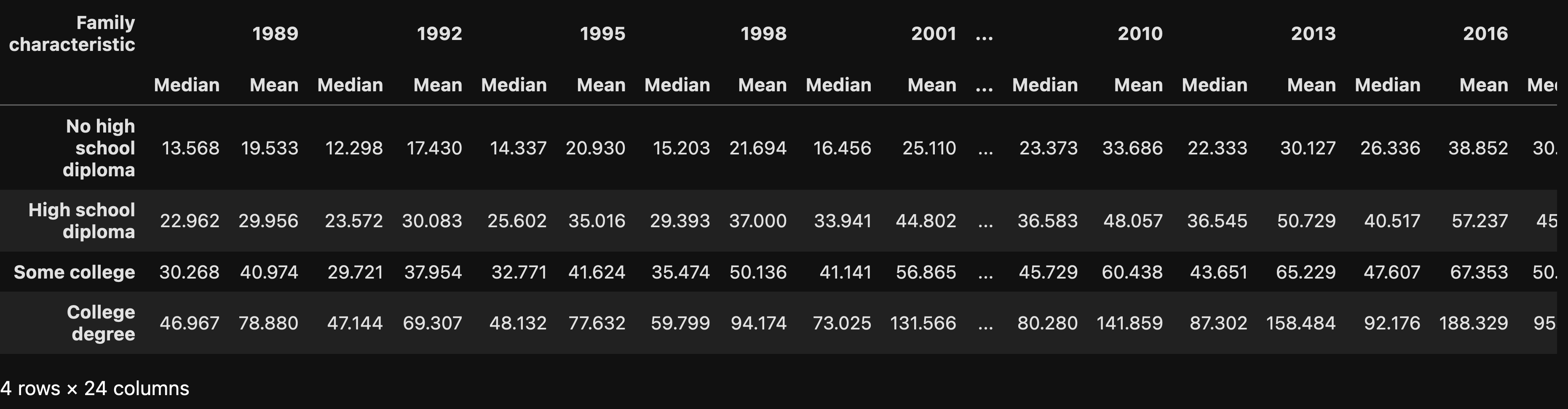
df = pd.concat(all_dfs, axis='columns')After doing all this, I got a data frame with 4 rows and 24 columns — 2 columns (mean and median) for each year of the survey.
Create a line plot with a separate line for each educational level, the x axis representing years, and the y axis showing median income in 2022 dollars. Which level of educational achievement appears to be improving its mean income level the most over the years?
Matplotlib is the best-known plotting library for Python, but whenever I can get away with it, I prefer to use the builtin Pandas plotting methods. They tend to be more limited, but they’re also (for me, at least) easier to work with, remember, and understand. (When things get more complex, or if I want the plot to look nicer, I use Seaborn instead.)
I wanted to see a line plot showing the median income for each educational level, with the x axis showing the progression of years. The idea is that we would be able to see whether, over the years, median income had improved or declined for each educational level.
We can always create a line plot from a data frame using the “plot.line” method. This gives us a separate line for each column, and uses the index for the x axis. While we could do this, it’ll give us a very weird, useless plot. Moreover, it’ll give us both the mean and the median, when we’re only interested in the median:
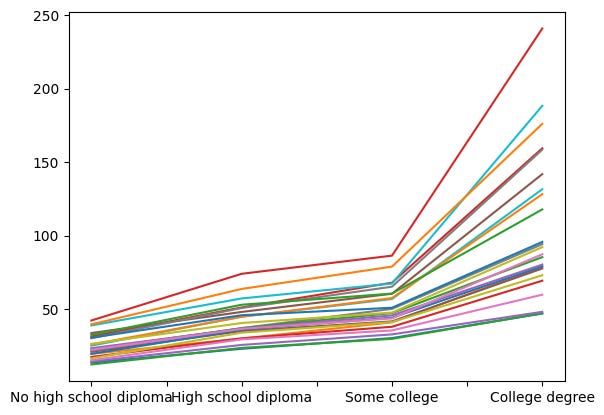
I removed the legend from the above plot, because it was covering most of the graph. But… this is totally useless.
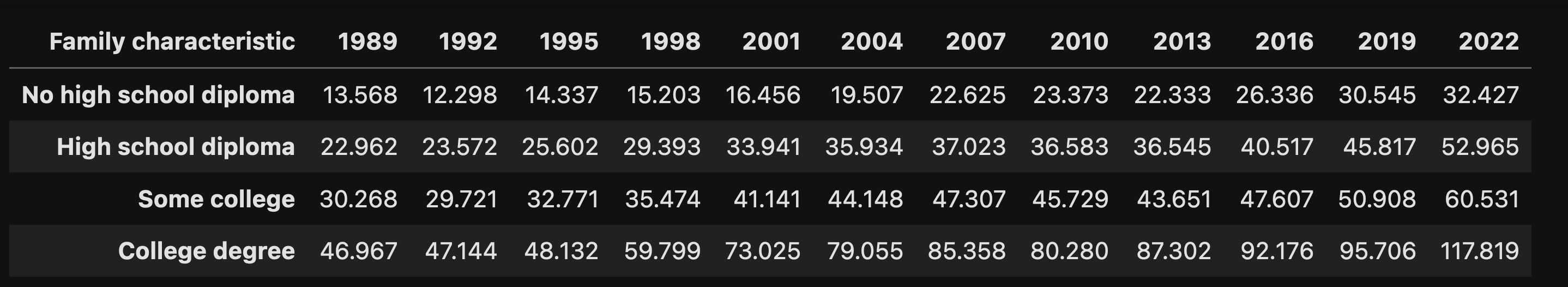
What we need to do is pull out only the columns with a “Median” value in the multi-index. Once again, we’ll turn to “xs”:
df.xs('Median', level=1, axis='columns')The above indicates that we want to select only those parts of the data frame for which level 1 (i.e., the second level) of the column multi-index has the value “Median”. The data frame that we get back lacks a mention of “Median”, just as the string you pass to “str.split” doesn’t appear in the list of strings that it returns. Here’s what I got back:
So we can just go ahead and plot now, right? No, not really — because we’ll again get a line for each column, and the x axis will be based on the index.
We need to transpose the data frame, swapping the two axes. We can do that with the “transpose” method, or its alias “T” (which doesn’t take parentheses). Then, with that in place, we can create the line plot:
df.xs('Median', level=1, axis='columns').T.plot.line()Here’s what we get:
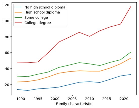
All educational levels have seen their median incomes rise over time. Not surprisingly, there is a strong correlation between the amount of education you got and your income. However, we see that in the last few years, the median income of college graduates has taken off, moving up and to the right very quickly, faster (it would seem from eyeballing it) than anyone else. People without a high-school education have seen their increases level off, becoming very close to flat.