

This week, we looked at data from a number of major stock-market indexes. The goals were not just to find out if the major drops we saw earlier this week were unusually large in historical terms, but also to see what connections we can find across the various indexes.

Data and six questions
There are a number of ways to download the data, and you'll get roughly the same information, in roughly the same format, no matter where you get it from. I personally went to investing.com (https://investing.com) where I signed up for a free account, went to the "major indices" page at https://www.investing.com/indices/major-indices , and downloaded a CSV file from January 1, 2005 through August 7, 2024 for the following indexes:
- DAX (Germany)
- Dow Jones Industrial Average (US)
- FTSE 100 (UK)
- NASDAQ (US)
- Nikkei 225 (Tokyo)
- S&P 500 (US)
- Shanghai Composite (China)
Here are the six tasks and questions that I posed for you based on this data. As usual, a link to the Jupyter notebook I used to put this together
Take the seven input CSV files, and turn them into a single data frame. The index of the data frame should be a two-part multi-index, with the first name of the filename on the outer layer and the date on the inner layer. We only care about the Date, Price, High, Low, Vol., and Change % columns.
For starters, I loaded Pandas. But I also loaded the os module from Python's standard library, since I'll use it in loading the files:
import pandas as pd
import os
I put all of the CSV files into a subdirectory called data under my Jupyter notebook's directory, and then made a list of those files:
filenames = ['DAX Historical Data.csv',
             'Dow Jones Industrial Average Historical Data.csv',
             'FTSE 100 Historical Data.csv',
             'NASDAQ Composite Historical Data.csv',
             'Nikkei 225 Futures Historical Data.csv',
             'S&P 500 Historical Data.csv',
             'Shanghai Composite Historical Data.csv']
Notice that it's totally OK for filenames to contain spaces. If you type the name on the command line, then you'll need to use quotes or backslashes – but in Python, where filenames are strings, it's easier to understand how we can include spaces.
Given those CSV files, how can we create a single data frame? The easiest way is to iterate over the filenames, creating one data frame from each. We can put those data frames into a list, and then use pd.concat to combine them.
However, there's a small snag, namely that we want to include to indicate from which file we took the data. Indeed, I want the resulting data frame to have a two-part multi-index, with the outer part indicating which index we're dealing with, and the inner part being the date of the reading.
I would normally use a list comprehension to read these files and create data frames from them, but adding the index name would complicate that. I thus decided to use a regular for loop, iterating over the list and creating a new data frame with each iteration. I created an empty all_dfs list, into which we can then append each of the data frames we create:
all_dfs = []

for one_filename in filenames:
    one_df = (pd
          .read_csv(os.path.join('data', one_filename),
                    usecols=['Date', 'Price', 'High',
                             'Low', 'Vol.', 'Change %'],
                    parse_dates=['Date'])
          .assign(source=one_filename.split()[0])
          .set_index(['source', 'Date'])
         )
    all_dfs.append(one_df)
Let's walk through the above code:
- First, we run
read_csv, reading in a filename. I use theusecolskeyword argument to indicate which columns I actually want in the resulting data frame, and theparse_datescolumn to indicate that theDatecolumn shouldn't be treated as a string, but rather as adatetimevalue. - Note that I use
os.path.jointo add an initial directory name (data) toone_filename, which is cleaner than using an f-string. - I then use the
assignmethod to add a new column to the data frame. I grab the first word fromone_filename, giving me a unique identifier that I can use, and assign it to all of the rows for thatsourcecolumn. - Having created a data frame from the CSV file, and then having added the
sourcecolumn from the filename, I then set the two-part index withset_index, passing a list of column names,sourceandDate. - Finally, I add the newly created data frame to
all_dfs.
When the loop has finished running, all_dfs is a list of data frames. We can then pass that to pd.concat, getting a single data frame back:
df = pd.concat(all_dfs)The result is a single data frame with a two-part multi-index on the rows, 28,637 rows, and 5 columns.
Modify the Change % to be a float column, rather than a string column. Modify Price, High, and Low, to be floats.
It's great that we managed to read the data into our data frame, but there is still work to be done. For example, the Change % column contains strings, even though we can actually work with the values if they're floats. In theory, we could use astype(float) on the column, getting a column of floats back – but we cannot do that with the values as they stand, because there is a % sign at the end of of each value.
Fortunately, Pandas comes with a lot of string functionality, all available via the str accessor. Many of the methods come from Python, but there are many that were inspired by other languages and frameworks. Even some of the Python methods have extra functionality, incorporating such features as regular expressions.
But to be honest, we don't need any of those things to turn the Change % column into a float dtype. We can use str.strip, a method well known to Python developers as able to remove leading and trailing whitespace from strings. It turns out that calling str.strip without any arguments is useful because we so often want to remove whitespace – but we can also pass a string argument to the method. In such a case, the characters in that string are all removed from the front and back of the string. For example, if I were to call str.strip('abc'), then the strings would not start or end with a, b, or c.
In this case, I'll run str.strip, passing it the single-character string '%' as an argument, to remove the % character from the end of the string. The resulting series of strings then contains strings that can be turned into floats with astype, which we then do, assigning the result back to df['Change %']:
df['Change %'] = (df
                  ['Change %']
                  .str.strip('%')
                  .astype(float)
                 )
We still have three other columns that we need to turn into float dtypes, as well. They all have the same problem, namely that the numbers contains commas every three digits – very nice for displaying numbers in a readable format, but not so good for calculations, or for using a float dtype.
We can solve this by invoking str.replace each of these columns, removing any commas. Then we can use astype(float) to get floats back. For example:
df['Low'] = df['Low'].str.replace(',', '').astype(float)This works, but I would rather not have three nearly identical assignments in a row. Maybe I can somehow do this in a loop?
I could, but I came up with an even wilder idea: I'll create a dict in which the keys are the column names, and the values are lambda expressions containing the combination of str.replace and astype. Even better, I can do this in a dict comprehension:
rewriting = {one_column :
               lambda df_: (df_[one_column]
                            .str.replace(',', '')
                            .astype(float))
             for one_column in ['Price', 'High', 'Low']
}
That's great, but what can I do with this dictionary? I can pass it to df.assign, which takes key-value pairs. However, we'll need to use ** to turn the dict we've created into those key-value pairs:
df = df.assign(**rewriting)This will invoke each of our lambda expressions on the associated columns, then assigning the new (float) values in place of the string values. And indeed, after running this, I can say:
df.dtypesAnd here's what I get:
Price       float64
High        float64
Low         float64
Vol.         object
Change %    float64
dtype: object
We're not there yet, but it's definitely progress.
Set the Vol. column to be an integer, and change its name to volume. Assume that B means "billion," M means "million," and K means "thousand".
This seemingly simple task turned out to be complex. Basically, I want to do the following:
- Grab the entire
Vol.column, except for the final character, and turn it into a float - Grab the final character from the
Vol.column, and use that to know the multiplication factor - Multiply the two numbers by one another, and put them into a new column called
volume.
My first attempt at doing this was a bit long and clumsy – which is normal when you're writing complex queries, and/or trying to do lots of things at once. Also, I often find it easier to break a problem apart into many small pieces, and then see if I can combine those pieces in smarter and better ways.
The first thing to do is define a dict that'll allow us to convert from the single-letter abbreviations to the numbers they represent:
factors = {'M':1_000_000, 'K':1000, 'B':1_000_000_000}The goal is for us to use map on a series of one-character strings taken from the end of the Vol. column, converting the letters M, K, and B into their respective numbers. We can pass map our factors dict, and it'll perform that conversion for us. Then we can multiply those values by the floats we get from Vol..
But first we have to actually turn Vol. into a float column we can do that with assign and lambda:
(
    df
    .assign(volume = lambda df_: df['Vol.'].str.slice(0, -1).astype(float))
)
The above returns our data frame with a new volume column of floats, taken from the Vol. column. As I indicated above, we want to take the values here and multiply them by the result of running map on the letters:
(
    df
    .assign(volume = lambda df_: df_['Vol.'].str.slice(0, -1).astype(float) *
                df_['Vol.'].str.get(-1).map(factors))
)
The result is a new volume column containing floats, the actual number of shares that were traded for each index.
However, we still have the original Vol. column. Let's use drop to remove it, making sure to specify axis='columns' so that Pandas looks for a column, rather than a row:
df = (
    df
    .assign(volume = lambda df_: df_['Vol.'].str.slice(0, -1).astype(float) *
                df_['Vol.'].str.get(-1).map(factors))
    .drop('Vol.', axis='columns')
)
We've now turned the original Vol. column into volume, and a string column into a float.
Create a data frame in which the columns are the index names, the rows are the dates, and the values are the percentage change in price from the previous day. But... you have to calculate the percentage change yourself, rather than use the data we got. (You can use it to double check your results, though.)
If we have a numeric series, and want to get the percentage change across the rows, then we can run pct_change. We can also run pct_change on a data frame; in such a case, we'll get one result per column.
The thing is, pct_change assumes that the data frame is sorted in ascending order, such that the earliest values are at the top and the latest values are at the bottom. If we're going to use pct_change on our data frame, we'll need to change that somehow.
One option is to sort the data frame by the index (probably using sort_index). But there is another way: We can tell pct_change not to compare each row with the one above it, but with 2 or 10 or 20 above it, by passing a value to the periods keyword argument. For example, if you have monthly sales totals in the rows of your data frame, you can ask pct_change to compare values from the same month in the previous year (e.g., August 2023 vs. August 2024) rather than the previous calendar month (e.g., July 2024 vs. August 2024).
If we pass periods=-1, then we'll still compare each row with its neighbor, but it'll be the following neighbor, rather than the preceding one:
(
    df['Price']
    .pct_change(periods=-1)
)
I must admit that I wasn't totally sure that Pandas would do the right thing here, calculating pct_change within each of the index names (i.e., the outer layer of the multi-index). But it worked like a champ, calculating the percentage differences for each day in each index.
The result, though, was a series with a two-part multi-index. I asked you to turn that into a data frame with index names across the columns and dates in the rows. I did that by using unstack, which does precisely what I just described, turning a long series into a less-long, but semi-wide data frame:
(
    df['Price']
    .pct_change(periods=-1)
    .unstack('source')
)
Note that I passed source to unstack as an argument, indicating that the outer layer (i.e., layer 0) of the multi-index should be moved into the columns, rather than the dates.
During which year and month did each index have its greatest gain and steepest percentage loss? How close was this week's drop?
Now that we know how to calculate the percentage changes, let's find the month in which each index had its greatest percentage gain and loss. First, we'll have to calculate the mean percentage change for each month; thankfully, because our index contains datetime values, we can use the resample method. resample is sort of like a groupby for datetime values, in that we have it run an aggregation method on the values. However, we can set the granularity of the time periods it uses.
In this case, we'll calculate the mean percentage change for each month. As of a recent version of Pandas, we can no longer use the granularity 1M to indicate one month; we must instead say either 1MS (start of one month) or 1ME (end of one month). I chose the latter.
My query thus looks like this:
(
    df['Price']
    .pct_change(periods=-1)
    .unstack(0)
    .resample('1ME')
    .mean()
)
The result is a data frame in which the index contains the final date of each month in the data set, from January 31st, 2005 through August 31, 2024. The latter is obviously (as of this writing) in the future, and simply means that all of the August, 2024 data will be put into that bin. (Sadly, this version of Pandas doesn't yet include functionality to tell you what stocks to pick over the coming weeks.)
How, though, can we get the greatest percentage gains and drops? I like to use the agg method, which lets us run multiple aggregation methods on a data frame. In this case, we'll want to run max and idxmax, as well as min and idxmin. Running just max and min would give us the largest gains and losses, but wouldn't tell us when those took place – hence, the addition of idxmax and idxmin:
(
    df['Price']
    .pct_change(periods=-1)
    .unstack(0)
    .resample('1ME')
    .mean()
    .agg(['max', 'idxmax', 'min', 'idxmin'])
)
To make it easier to read, I transposed the result (with T), and this is what we get:
               max               idxmax       min               idxmin
source
DAX       0.007886  2009-04-30 00:00:00 -0.042801  2005-01-31 00:00:00
Dow       0.217157  2024-07-31 00:00:00 -0.012596  2024-08-31 00:00:00
FTSE      0.006011  2020-11-30 00:00:00 -0.034847  2005-01-31 00:00:00
NASDAQ    0.007113  2020-04-30 00:00:00 -0.049023  2005-01-31 00:00:00
Nikkei    0.026283  2009-03-31 00:00:00 -0.021556  2024-08-31 00:00:00
S&P       0.005874  2020-04-30 00:00:00 -0.030208  2005-01-31 00:00:00
Shanghai  0.011053  2006-12-31 00:00:00 -0.013998  2016-01-31 00:00:00
We can see that July of 2024 – just last month! – ended the biggest run-up in the Dow Jones Industrial Average, an index that is simultaneously famous and dismissed by many of the financial journalists I read. We can see that the others rose at different times, although the S&P and NASDAQ had big runups in April of 2020 – I'm guessing just after massive drops due to the pandemic.
Many of the largest drops appear to be on January 31st, 2005; I'm not sure what happened there, but it could just be an artifact of the data starting in January 2005, and thus not having much to go on. We do, however, see that the Nikkei index from Japan and the Dow both had their biggest-ever percentage drops this month. We're only a week or so into the month, so there's still time to recover.
How closely correlated are the daily percentage changes in different indexes? Show the correlations, showing any correlation about +0.75 in red, and any under +0.25 in blue. (There aren't any negative correlations with this data, so we don't have to worry about that.) Are changes in US markets more highly correlated with each other than with non-US markets?
After calculating the percentage change, we can then run the corr method on our data frame. This returns a new data frame, one in which the original's columns are both the column and index. The idea is that we can then see, on a scale of -1 (100% negative correlation) to 0 (no correlation) to +1 (100% positive correlation) the relationships between the columns:
(
    df['Price']
    .pct_change(periods=-1)
    .unstack(0)
    .corr()
)
The result:
source         DAX       Dow      FTSE    NASDAQ    Nikkei       S&P  Shanghai
source
DAX       1.000000  0.086478  0.578778  0.827575  0.318786  0.813472  0.185111
Dow       0.086478  1.000000  0.016123  0.159893  0.091386  0.158906  0.006728
FTSE      0.578778  0.016123  1.000000  0.409673  0.349620  0.455120  0.206568
NASDAQ    0.827575  0.159893  0.409673  1.000000  0.227810  0.944094  0.154431
Nikkei    0.318786  0.091386  0.349620  0.227810  1.000000  0.250709  0.242580
S&P       0.813472  0.158906  0.455120  0.944094  0.250709  1.000000  0.172233
Shanghai  0.185111  0.006728  0.206568  0.154431  0.242580  0.172233  1.000000
As you can see the diagonal is all 1.0 values, because (by definition) a column is 100% positively correlated with itself. But which are highly correlated with one another, and which are very loosely correlated? It's hard to see in such output.
Fortunately, Pandas has a style object, on which we can run methods to change the color of the cells. One of those methods is highlight_between, in which we can tell Pandas that if a cell's values are between a certain minimum and maximum, it should set the background to be a particular color. In our case, I'll say:
(
    df['Price']
    .pct_change(periods=-1)
    .unstack(0)
    .corr()
    .style.highlight_between(left=-1, right=0.25, color='blue')
    .highlight_between(left=0.75, right=0.99, color='red')
)
Notice that I set the max to be 0.99, rather than 1, so as not to highlight the diagonal (which will always be 1.0). The result:
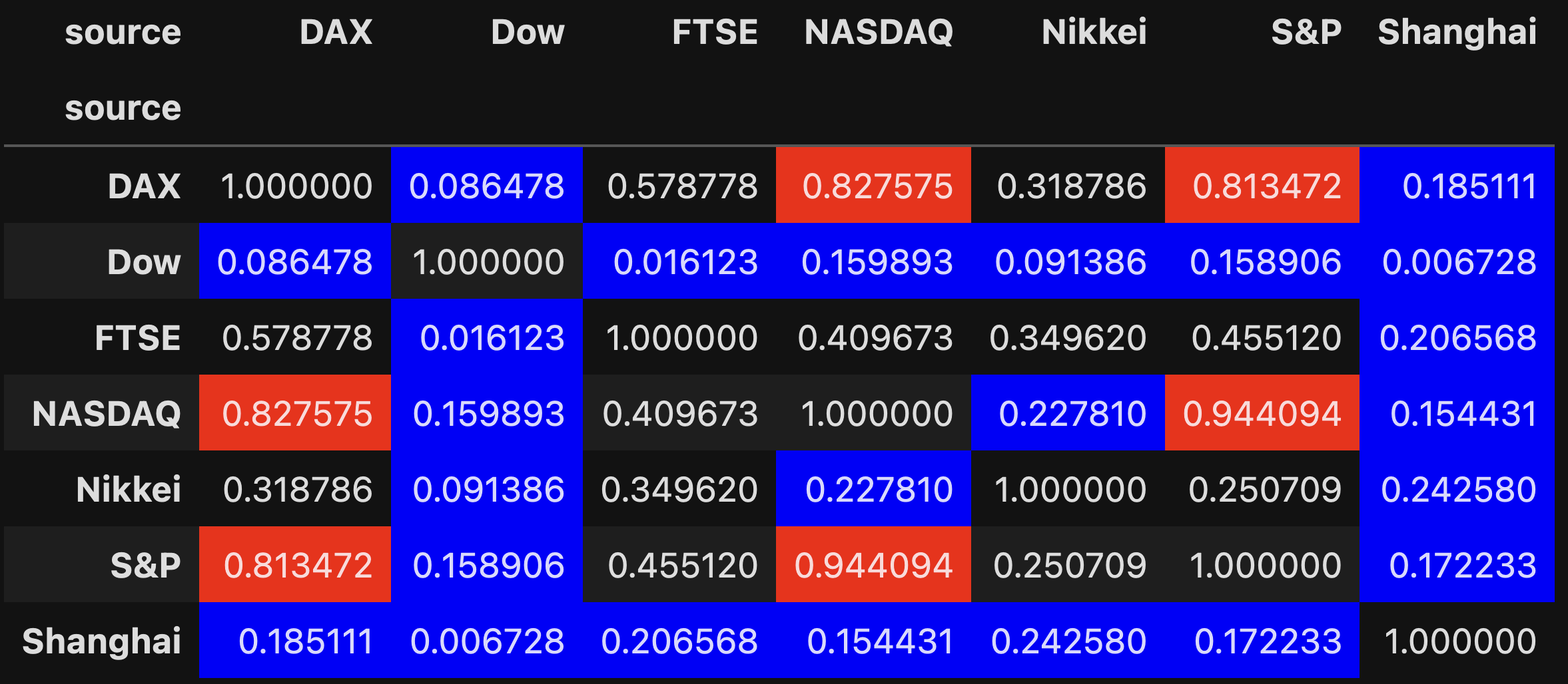
We can see that the S&P and NASDAQ are very closely correlated, and that they're both pretty closely correlated with the German DAX. There is almost no correlation between the Dow and other indexes, which might indicate why so many people dismiss it as irrelevant. The Shanghai index also appears to have very low correlation with the others.
I hope that you enjoyed this week's edition! Here's a link to the Jupyter notebook I used for this week: https://drive.google.com/file/d/1FQiIjb4c_INgXhNKryq_gCCNW9M2veq0/view?usp=sharing
I'll be back next week with more Pandas puzzles based on current events.
Reuven