


Four (!) administrative notes:
- This Sunday, I’ll be holding Pandas office hours, open to all paid subscribers and members of my membership program at https://LernerPython.com . I’ll send e-mail in the coming day with the full info and Zoom link.
- Next week, I’ll be moving Bamboo Weekly from Substack to another platform, Ghost. Things should go pretty smoothly, and I expect to get a new issue out on Wednesday of next as usual. But there will likely be some hiccups, and I’ll appreciate whatever bug reports you can send me.
- If you’re new with Python and Pandas, then you might want to check out my Python Data Analytics Bootcamp (https://PythonDAB.com/), which starts in two weeks. Check out the Web site for more info, or join me at a free webinar and explanation at https://store.lerner.co.il/pythondab-spring-2024 .
- If you have read and enjoyed Pandas Workout, my book with 200+ exercises in Pandas, would you please add a review on Amazon? Such reviews really do help new people to find the book. Note: You don’t have to buy the book on Amazon to review it there.
And now, back to this week’s solutions
Like many nerds, I’ve long been interested in space and space exploration. You probably won’t be surprised to hear that when I was little, I subscribed to “Odyssey,” a children’s magazine about astronomy. I read their articles about planets, galaxies, asteroids, and everything else, including the then-new Voyager 1 and 2 spacecraft. I even wrote several book reviews for Odyssey — my first paid writing gig!
While we have long associated the United States (and NASA) with cutting-edge space exploration, other countries have been increasingly daring and impressive on this front. In particular, China is pushing forward into space, most notably and recently with the landing of Chang'e 6 (https://en.wikipedia.org/wiki/Chang%27e_6) on the far side of the moon. The plan is for Chang’e 6 not only to land there, but to extract soil samples and send them back to Earth via a spacecraft orbiting the moon. That’s pretty darned impressive.
This week, I thought it might thus be interesting to look at the history of moon missions. And while the glory days, as we think of them, took place in the 20th century, there was enough data to play with just from this century.
By the way, if you’re also into space exploration, I recommend the Apple TV+ series “For All Mankind,” which shows an interesting alternative history.
Data and six questions
This week’s data was from Wikipedia, which conveniently has a page dedicated to all of the moon missions:
https://en.wikipedia.org/wiki/List_of_missions_to_the_Moon
That page contains several HTML tables, including one containing information about moon missions in the 21st century. That table will be our data source for this week.
Here are my detailed answers and explanations for all of the questions; a link to download my Jupyter notebook is below.
This week's learning goals include scraping HTML, cleaning data, working with indexes and multi-indexes, and working with dates and times.
I’ll be back tomorrow with my complete answers, including a downloadable version of my Jupyter notebook.
Here are this week's six tasks and questions:
From the Wikipedia page (https://en.wikipedia.org/wiki/List_of_missions_to_the_Moon), turn the table of 21st-century missions into a data frame. In the HTML table, the final row for each mission describes that mission; remove all of those descriptive rows. Set the index to be the mission + spacecraft.
Before doing anything else, we need to load up Pandas:
import pandas as pdWith that in hand, I asked you to retrieve data from Wikipedia. There are a variety of Web-scraping techniques and libraries out there, but my favorite is the “read_html” method in Pandas, which returns a list of data frames, one for each HTML table at the URL in question.
The list of data frames is apparently in the same order as they appear on the stage. This means that the first data frame represents the first table, index 1 represents the second, and so forth. Don’t forget that Wikipedia uses tables for a variety of purposes, including tables of contents. It turns out that the table we want, containing data about moon missions in the 21st century, is at index 1. We can thus retrieve it as follows:
url = 'https://en.wikipedia.org/wiki/List_of_missions_to_the_Moon'

df = (
    pd
    .read_html(url)
    [1]
)
If you look at the data frame we get from this scraping, you’ll see how hard Pandas (and/or the underlying scraping library) is working to turn the HTML into a data frame. For example, the “Mission” column in the original data frame covers two columns. As a result, we end up with two columns, one called “Mission” and the second called “Mission.1”. For now, we’ll set the data frame’s index to be “Mission” using “set_index”, but we’ll come back to that and change it soon enough:
url = 'https://en.wikipedia.org/wiki/List_of_missions_to_the_Moon'

df = (
    pd
    .read_html(url)
    [1]
    .set_index('Mission')
)
Remember that “set_index”, like most Pandas methods, returns a new data frame reflecting the requested changes, rather than modifying the data frame on which it’s running.
Next, I decided to clean up the “Operator” column using “assign”, along with a lambda, “str.replace”, and a regular expression:
url = 'https://en.wikipedia.org/wiki/List_of_missions_to_the_Moon'

df = (
    pd
    .read_html(url)
    [1]
    .set_index('Mission')
    .assign(Operator=lambda df_: df_['Operator'].str.replace(r'\[\w+\]', '', regex=True))
)
Because I’m passing the “Operator” keyword argument to “assign”, and because the input is also coming from “Operator”, we’re effectively modifying and updating the column. The update here is to remove the “[1]” style footnotes that appear in the column, thus allowing us to compare notes on the “Operator” column. The regular expression is
\[\w+\]Which means:
- A literal [ character
- One or more letters, digits, or _ characters
- A literal ] character
In other words, we’re looking for one or more letters and digits inside of [], and we’ll use “str.replace” to replace them with the empty string — meaning, we’ll remove them.
With this query done, we can start to do the harder thing, namely remove the mission description from the table.
To be honest, I spent a ton of time figuring out how to do this. In the end, I decided that maybe this was one of those times when iterating isn’t a totally bad thing to do; I iterated over the data frame’s multi-index, giving me smaller data frames with each iteration. I could then grab all of the rows except the final one using `.iloc`, concatenate them onto a list, and then finally call “pd.concat” to join them together:
output = []

for index, one_index in enumerate(set(df.index)):
    mini_df = df.loc[one_index]
    mini_df = mini_df.iloc[:-1]
    output.append(mini_df)

df = (pd
      .concat(output)
      .set_index(['Mission.1', 'Spacecraft'])
     )
The good news? It worked. The bad news? I felt like I was missing something, that perhaps I could do this better, or more elegantly. Iterating is almost always an indication that you’re doing something wrong.
Then I looked at the data more closely, and saw that because the description stretches across all of the rows, Pandas treats it as identical values in each of the columns. That is, the “Spacecraft” and “Launch date” columns don’t contain info about the spacecraft and launch dates. Rather, they contain text — the same text — describing the mission. I thus realized that I could greatly simplify my code by just removing any row in which the “Spacecraft” and “Launch date” columns contained identical data:
df = (
    df
    .loc[df['Spacecraft'] != df['Launch date']]
    .set_index(['Mission.1', 'Spacecraft'])
)
I used “%%timeit” to compare how long each of these took. It wasn’t a huge difference — so the reason to use the second query isn’t speed, but rather readability and maintainabilty. Which, after all, should almost always be our primary consideration.
In both cases, we end up with a data frame with a two-part multi-index, 78 rows, and 5 columns.
Turn the "Launch date" column into a datetime column.
All of the columns can and should be textual, meaning that they’ll have a dtype of “object”, except for the “Launch date” column. Pandas interpreted it as a string column, but in order to get the most out of it, we’ll want to give it a dtype of “datetime”.
In theory, we can do that by calling “pd.to_datetime” on the column. The input is a series of strings, the output is a series of datetimes, and we can just assign that back to the same column.
However, there’s a problem with this approach, namely that the strings contain footnotes, much as we saw with the “Operator” column above. Here, though, I’ll just look for \d+ (i.e., one or more digits).
I can run my column through “str.replace”, and then I get a new column back. It’s on this new column that I want to run “pd.to_datetime”. But how can I do that? Of course, I could just run the function on the output from “str.replace”, and assign that back to the original column.
But this is actually a good place to use “pipe”. If you have a function that takes a series as an argument, then you can pass it as an argument to “pipe”. Your function will be invoked with the series as an argument, letting you use it in method chaining:
df['Launch date'] = (df['Launch date']
                     .str.replace(r'\[\d+\]', '', regex=True)
                     .pipe(pd.to_datetime)
                    )
By the way, we could have used “assign” here as well, except for the fact that the column name contains a space character. I decided that we could just use “real” assignment. Another option would have been to rename the column, or assign to a new name and remove the old one.
How many missions included at least one spacecraft that's identified as "cubesat or similar"?
The table listing 21st-century moon missions showed that a number of the spacecraft were “cubesat or similar,” meaning very small spacecraft. How many missions included at least one such spacecraft?
To find that out, I first used “reset_index” to move just the outer layer (“Mission.1”) of our multi-index back to the main data frame. I then selected just that column, meaning that I now had a series:
(
    df
    .reset_index(level=0)
    ['Mission.1']
)
Next, I used “filter” to keep only those rows in which the index began with the cubesat symbol:
(
    df
    .reset_index(level=0)
    ['Mission.1']
    .filter(regex='^⚀', axis='rows')
)
Finally, I invoked “value_counts” to learn not just how many missions included at least one cubesat, but how often they have been used:
(
    df
    .reset_index(level=0)
    ['Mission.1']
    .filter(regex='^⚀', axis='rows')
    .value_counts()
)
Here are the results I got:
Mission.1
Artemis 1                10
CAPSTONE                  1
Lunar Flashlight          1
Peregrine Mission One     1
IM-1                      1
Chang'e 6                 1
Name: count, dtype: int64
How many launches were there per 5-year period? Create a bar plot showing the number. Do we see any change over time? (If a mission contains multiple spacecraft, you can count each one separately.)
To find out how many launches there were, we can use the “count” method. But to count how many launches there were during each 5-year period, we’ll need to use a “groupby” operation. Normally, “groupby” operates on the unique values in a categorical column. However, using “Grouper”, we can not only operate on a datetime column, but we can specify the frequency of sampling.
For Grouper to work, we need to specify which column we want to work with, and the frequency we want to group it on. In this case, I’ll ask to operate on the “Launch date” column, and I’ll specify “5YE” (short for end-of-5-year periods):
(
    df
    .groupby(pd.Grouper(key='Launch date',
                        freq='5YE'))['Outcome'].count()
)
The above query gave the following result:
Launch date
2001-12-31     1
2006-12-31     3
2011-12-31    13
2016-12-31     6
2021-12-31    14
2026-12-31    41
Freq: 5YE-DEC, Name: Outcome, dtype: int64
It certainly looks like an upward trend (no pun intended), but let’s plot it to be sure, using “plot.bar”:
(
    df
    .groupby(pd.Grouper(key='Launch date',
                        freq='5YE'))['Outcome'].count()
    .plot.bar()
)
I got the following result:
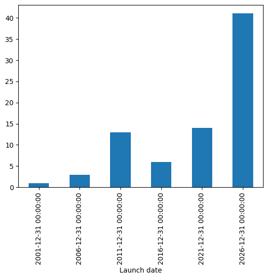
It’s not a constant upward trend, but we can definitely see a huge increase in just the most recent five years.
Create a stacked bar plot, showing how many spacecraft were launched to the moon by NASA, CNSA (China National Space Administration), ISRO (Indian Space Research Organization), or JAXA (Japan Aerospace Exploration Agency) in each year.
I loved stacked bar plots; I find them both attractive and useful, allowing us to compare values as they change over time, while also breaking down their individual components. For this exercise, I asked you to create a stacked bar chart, showing us how many launches we had per year from each of NASA, CNSA, ISRO, and JAXA.
I started by using “loc” and “lambda”, along with “isin”, to keep only those rows where those four operators were named:
(
    df
    .loc[lambda df_: df_['Operator'].isin(['NASA', 'CNSA',
                                           'ISRO', 'JAXA'])]

)
With that in place, I thought it might be easiest to create a pivot table in which the year of the launch date would be the rows, the operators would be the columns, and we could invoke the “count” aggregation method. I invoked “pivot_table” in order to create that:
(
    df
    .loc[lambda df_: df_['Operator'].isin(['NASA', 'CNSA',
                                           'ISRO', 'JAXA'])]
    .pivot_table(index=df['Launch date'].dt.year,
                 columns='Operator',
                 values='Outcome',
                 aggfunc='count'
                )
)
Finally, I invoked “plot.bar” with the stacked=True option:
(
    df
    .loc[lambda df_: df_['Operator'].isin(['NASA', 'CNSA',
                                           'ISRO', 'JAXA'])]
    .pivot_table(index=df['Launch date'].dt.year,
                 columns='Operator',
                 values='Outcome',
                 aggfunc='count'
                )
    .plot.bar(stacked=True)
)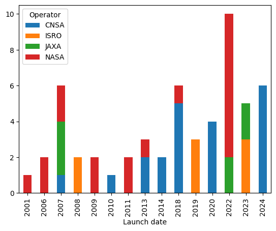
We can see that CNSA has definitely be doing more and more moon missions in the last decade or so. Japan, about whose space agency I know little, has been doing a bit in the last few years, as well.
For each operator, what proportion of launched spacecraft had an outcome that does not include the word "failure"?
To find those rows in which the “Outcome” column does not contain “ailure” (i.e., the latter part of “Failure” and “failure”, we can use .loc, along with ~ to negate the results:
(
    df.loc[lambda df_: ~(df_['Outcome'].str.contains('ailure'))]
)
But I don’t want to know how many rows there are. Rather, I want to know how many there are per operator. For this, we add a “groupby”:
(
    df.loc[lambda df_: ~(df_['Outcome'].str.contains('ailure'))]
    .groupby('Operator')['Outcome'].count()
)
Then we divide the series we just got by the overall count of launches by the operator. In other words, we calculate the success rate for that operator, measured by spacecraft:
(
    df.loc[lambda df_: ~(df_['Outcome'].str.contains('ailure'))]
    .groupby('Operator')['Outcome'].count()
    /
    df.groupby('Operator')['Outcome'].count()
)
We then remove the NA values, and finish by invoking “sort_values” in reverse:
(
    df.loc[lambda df_: ~(df_['Outcome'].str.contains('ailure'))]
    .groupby('Operator')['Outcome'].count()
    /
    df.groupby('Operator')['Outcome'].count()
).dropna().sort_values(ascending=False)
And here are the results:
Operator
ASI                                                     1.000000
CAS                                                     1.000000
UAESA/MBRSC                                             1.000000
Tomy/JAXA/Dodai                                         1.000000
Tomy / JAXA / Doshisha University                       1.000000
SUPARCO                                                 1.000000
LuxSpace                                                1.000000
Lockheed Martin                                         1.000000
KARI                                                    1.000000
UNAM                                                    1.000000
Intuitive Machines                                      1.000000
Fluid & Reason                                          1.000000
ESA                                                     1.000000
Deep Space Exploration Laboratory (DSEL, Tiandu Lab)    1.000000
CMU                                                     1.000000
CNSA                                                    0.952381
ISRO                                                    0.875000
JAXA                                                    0.857143
NASA                                                    0.736842
Name: Outcome, dtype: float64
Don’t forget that some of these operators with 100% records only launched one mission. So they would either be 100% or nothing at all. Also, measuring by spacecraft might not be the fairest thing, since one launch might include a large number of spacecraft. But it’s clear that moon landings and exploration are starting to gear up, and NASA isn’t the only game in town for a change.
I hope that you enjoyed this! Here’s a link to my Jupyter notebook: https://drive.google.com/file/d/1llX7iiSdQJL9m2EfbXTdExxn_2w9SGCE/view?usp=drive_link
I’ll be back on Wednesday — from our new home on Ghost, if all goes well — with more challenges in Pandas from current events.
Reuven