


[Note: We'll be holding Pandas office hours this coming Sunday at 17:00 in Israel, aka 10 a.m. Eastern. On Friday, I'll send full Zoom info to paid subscribers. Come with any and all Pandas questions!]
This week, we looked at China's exports – how much have their exports to the United States changed over the last two years, and to what countries are they exporting instead of the United States? The backdrop for this is President Donald Trump's tariffs, and particularly his tariffs on Chinese imports to the United States, which he imposed to reduce the trade deficit between the two countries.
This week's topic was inspired by a recent article in the Economist, which indicated that while the US is importing less from China than it used to, China has more than made up for this change by exporting to other countries (https://www.economist.com/finance-and-economics/2025/09/09/chinese-trade-is-thriving-despite-americas-attacks?giftId=1d26bcbb-40c2-407c-8079-9071ee03068e&utm_campaign=gifted_article).
This week, we'll look at Chinese government statistics from the last three years. Is trade between China and the United States declining? What countries are importing more from China than they used to, and which are importing less? And do any countries have a trade surplus with China?
Data and five questions
This week's data comes from the China Customs official Web site, where they post a variety of monthly reports, at http://english.customs.gov.cn/statics/report/monthly.html . Because the most recent data for 2025 is from August, and because I want to look at trade on a country-by-country basis, I want you to download the Excel files for August 2025, 2024, and 2023. These are available by choosing each year, selecting "Imports and Exports by Country (Region) of Origin/Destination," and downloading the file via the link at the bottom of the page.
Learning goals for this week are reading from multiple Excel files, filtering, regular expressions, multi-indexes, window functions, styling, and plotting with Plotly.
Paid subscribers to Bamboo Weekly, including subscribers to my LernerPython membership platform (https://LernerPython.com), can download the data files via a link at the bottom of this message. You can also download my Marimo notebook and get one-click access to work through it in your browser. Paid members also see all questions and answers (not just the first two), and are invited to monthly office hours.
Here are my five questions and tasks for this week, along with my solutions and explanations:
Combine the three Excel files into a single Pandas data frame. The country names should be the data frame's index. We only need two columns from each data file, "Imports" and "Exports" for 8 (i.e., August) of each of the three years. The resulting data frame should have six columns with a two-level multi-index; the outer level will be the year, and the inner level will be either "Imports" or "Exports". Remove leading/trailing whitespace from each index entry.
Before doing anything else, I loaded up Pandas:
import pandas as pd
Next, I had three Excel files, one for each of the years (2023, 2024, and 2025). Loading a single file into a data frame is fairly straightforward, using the read_excel method. I passed the header keyword argument to indicate that rows 3-4 (what Excel would see as rows 4-5, due to Python's zero-based indexing) should contain the headers, and that column 1 should be used as the index.
Specifying two rows, rather than one, for header meant that the resulting data frame would have a two-part multi-index on the columns. We'll get back to that in just a little bit.
When I tried to load the data that way, I quickly discovered that there was still at least one major issue: I couldn't convert the data to float values, because there were '-' characters to indicate missing data. In Pandas, we use NaN to indicate missing data. How could I tell Pandas that it should treat '-' cells as NaN? With the na_values keyword argument to read_excel, which indicates which values (yes, you can pass more than one) should be treated as NaN. I got:
(
    pd
    .read_excel(one_filename,
               header=[3, 4],
               index_col=1,
               na_values=['-'])
)
With the data frame loaded into Pandas, I needed to perform some additional surgery on it. First, I wanted to choose only the two columns for imports and exports in August. That meant not only specifying the outer column names of 'Imports' and 'Exports', but also the inner values. Those inner values might have looked like integers, but they were actually strings, '8', so trying to retrieve them with an integer failed.
I can request a column from a data frame with []. How can I specify a column that has a two-level multi-index? If I use a list of lists, then Pandas thinks I want to use fancy indexing to retrieve more than one column. And I do want more than one column, so I will need a list of lists... but what will the inner list contain?
Pandas allows us to specify multiple segments of a multi-index using a tuple. I can thus say ('Imports', '8') to indicate that the outer layer should be 'Imports', and that the second (inner) layer should be '8'. The result of this query is a two-column data frame:
(
    pd
    .read_excel(one_filename,
               header=[3, 4],
               index_col=1,
               na_values=['-'])
    [[('Imports', '8'), ('Exports', '8')]]

)
I did a bit more housecleaning on the data:
- I invoked
astype(float)on the data frame. Normally, I would useastypeon a specific column, but all of the values in this (now two-column) data frame should be floats. Thanks to passingna_values=['-'], missing values were treated asNaN, which meant thatastypehandled them without any problems. - It turns out that the index column for a number of rows was
NaN, that these rows were unneeded, and that keeping these rows caused problems down the road. So I usedlocwithlambda, invokingnotnaon the data frame's index. The result was that only those rows with a non-NaNindex remained. - There was no reason to keep around the inner layer of the multi-index. I invoked
droplevel, which removed that inner layer. - I wanted to remove leading and trailing whitespace from country names in the index. To do this, I used
rename, passing it the keyword argumentindexand giving it the functionstr.strip. The result of invoking this function was then assigned back to be the index.
Here's the code to do all of this:
(
    pd
    .read_excel(one_filename,
               header=[3, 4],
               index_col=1,
               na_values=['-'])
    [[('Imports', '8'), ('Exports', '8')]]
    .astype(float)
    .loc[lambda df_: df_.index.notna()]
    .droplevel(1, axis='columns')
    .rename(index=str.strip)
)
The above code is just fine for reading in a single Excel file, and getting a data frame based on it. However, we have three files, and I wanted to keep them together.
I put the above code inside of a list comprehension, iterating over the filenames that matched a "globbing" pattern. I used glob.glob to get a list of files matching that pattern, then iterated over those names, assigning one_filename to each filename, one at a time. The result was a list of data frames:
import glob

pattern = '/Users/reuven/Downloads/202[345]-08_M122USD*xls'

[(
      pd
      .read_excel(one_filename,
                 header=[3, 4],
                 index_col=1,
                 na_values=['-'])
      [[('Imports', '8'), ('Exports', '8')]]
      .astype(float)
     .loc[lambda df_: df_.index.notna()]
     .droplevel(1, axis='columns')
     .rename(index=str.strip)
      )
    for one_filename in glob.glob(pattern)
]
How can I turn this list of data frames into one, single data frame? I've often used pd.concat along with a list comprehension for these purposes. pd.concat takes a list of data frames and combines them into a single data frame, which it returns.
However, by default pd.concat joins them together vertically. And in this case, we actually want to join them horizontally, such that our three two-column data frames produce a single six-column data frame. To do that, we need to say axis='columns'. pd.concat will then join them across the rows, finding where those match up. Fortunately, the list of countries and territories is the same across the three files I asked you to load, allowing us to compare the three most recent years.
We do need one more thing, though: pd.concat could combine all three of the data frames into a single one. But each of the original data frames has the same column names, 'Imports' and 'Exports'. We'll need to distinguish between each year's data. To do that, we can pass the keys keyword argument to pd.concat. This forces the creation of a multi-index in the columns, using the keys that we provided.
Note that I passed the years as strings, rather than as integers. This was to avoid Pandas warnings about using integers as column names.
So we started with three multi-indexed data frames, flattened their columns, and then reintroduced a multi-index when concatenating them.
The final query looks like this:
pattern = '/Users/reuven/Downloads/202[345]-08_M122USD*xls'

df = pd.concat([(
                pd
                .read_excel(one_filename,
                           header=[3, 4],
                           index_col=1,
                           na_values=['-'])
                [[('Imports', '8'), ('Exports', '8')]]
                .astype(float)
               .loc[lambda df_: df_.index.notna()]
               .droplevel(1, axis='columns')
               .rename(index=str.strip)
                )
              for one_filename in glob.glob(pattern)],
         axis='columns',
         keys=['2023', '2024', '2025']
)
The resulting data frame contains 273 rows and 6 columns.
Using Plotly, create a line plot showing how much China exported to the US in August of each of these three years, and how much the US exported to China during those same three years. What trends do you see, if any? By what percentage did trade in each direction change over these three years? Display the numbers as percentages.
Given that the data frame's index contains country names, I retrieved the row for the United States with loc:
(
    df
   .loc['United States']
)
Because that returned a single row, Pandas produced a series rather than a data frame. However, this series had a two-level multi-index, coming from the two-level multi-index on the data frame's columns. The inner level of the multi-index contained the strings 'Imports' and 'Exports'. I wanted to compare imports vs. exports for each year, both numerically and graphically.
To do that most easily, I used unstack to move the inner level of the series multi-index to a data frame. This left me with a data frame whose three rows contained years, with two columns, 'Imports' and 'Exports':
(
    df
   .loc['United States']
    .unstack(level=1)
)
To get a line plot using Plotly Express, I could invoke px.line on the result of the query. However, I like to use method chaining whenever possible, and the pipe method allows us to turn a function into a method. I could thus say:
from plotly import express as px

(
    df
   .loc['United States']
    .unstack(level=1)
    .pipe(px.line)
)
In the above code, pipe passes the data frame from unstack to px.line as an argument. It then creates the plot.
However, I asked you to set the title of the plot. That requires passing an argument to px.line. How can we do that?
One way would be to use lambda inside of pipe, which I've often done before:
(
    df
   .loc['United States']
    .unstack(level=1)
    .pipe(lambda df_: px.line(df_,
                             title='US/China trade'))
)
However, I recently discovered that there's an easier way: pipe takes both *args and **kwargs , and passes them along to the function we pass for invocation. In other words, I don't need to use lambda, because I can just say:
(
    df
   .loc['United States']
    .unstack(level=1)
    .pipe(px.line, title='US/China trade')
)
This is true for any other arguments we might wish to pass. So yes, lambda is still useful in pipe, but less crucial than I used to believe.
The resulting plot looks like this:
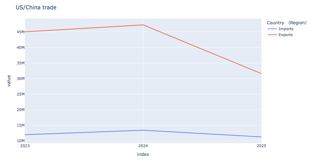
We can see that exports (from China to the US) were relatively steady, or even increased a bit, from 2023 to 2024. But from 2024 to 2025, we see a dramatic drop. The number of imports (from the US to China) also dropped quite a bit, reflecting the pain that US exporters are feeling about a market to which they had sold for many years.
Let's put some numbers to that: By how much did trade between the US and China change over the last few years? To answer that question, we can use a built-in window function, pct_change.
This query starts the same as the above one. But instead of plotting, I invoked pct_change to find the change from each year to the next. The result from pct_change is a data frame with the same index and column names as the data frame on which it was invoked; the first row contains all NaN values, because it is the basis for comparison. I invoked dropna to remove it. The result:
(
    df
   .loc['United States']
    .unstack(level=1)
    .pct_change()
    .dropna()
)
This gives us the answers we want, but I asked to style it a bit more nicely. I used the style object that every data frame has, then invoking format. By passing a format string (i.e., one that can be passed to str.format), I was able to indicate that all values should be displayed with one digit after the decimal point, and then as a percentage (i.e., '.1%'):
(
    df
   .loc['United States']
    .unstack(level=1)
    .pct_change()
    .dropna()
    .style.format('{:.1%}')
)
The result:
Country (Region)    Imports	Exports
2024	            12.2%	4.9%
2025	            -16.0%	-33.1%
In other words, imports from the US to China grew by 12.2 percent from 2023 to 2024. But they then dropped by 16 percent from 2024 to 2025. That's pretty steep!
Things are even worse on the export side: China's exports to the US grew by nearly 5 percent from 2023 to 2024. But in the last year, they dropped by about one third.
Trump has long (even before entering office) been opposed to trade, and especially to trade deficits. So he might see this as a win. However, such a huge drop in US imports from China likely means that products are either less easily available, more expensive, or both. And these numbers show why so many US exporters are looking for new international markets, since China has become a much harder sell.