


Earlier this week, JetBrains (makers of the popular PyCharm IDE, among other things) and the Python Software Foundation released the results from their latest Python usage survey. This is an annual attempt to find out who is using Python, what they're using it for, and what parts of the language they're using.
There are blog posts summarizing the survey from the PSF (https://pyfound.blogspot.com/2025/08/the-2024-python-developer-survey.html) and also from JetBrains, in a guest blog post from Michael Kennedy (https://blog.jetbrains.com/pycharm/2025/08/the-state-of-python-2025/).
I saw the postings about the survey and decided that since we're all Python people here, and we're using Python to analyze data, maybe we should use Python to analyze data about Python? Better yet, we'll use Python and Pandas to analyze data about Python and Pandas.
Data and five questions
The home page for this year's survey results is at https://lp.jetbrains.com/python-developers-survey-2024/. To download the raw data, go to the bottom of the page. and click on the yellow "download survey's raw data" button. That'll take you to a shared Google Drive folder, from which you can download the survey data (in a zipped CSV file), along with a data dictionary, the survey itself, and some other related information.
We'll work with the CSV data file to answer this week's questions.
Learning goals include working with NaN values, PyArrow, filtering and renaming columns, formatting strings, and plotting with Plotly.
Paid subscribers, including subscribers to my LernerPython+data program, can download the file from the end of this message.
Here are the five tasks and questions; I'll be back tomorrow with my solutions and extended explanations:
Read the data into a Pandas data frame. Why do get a warning regarding dtypes using the default CSV-loading engine? Why does this warning go away if we use the PyArrow engine? For what percentage of respondents is Python their main programming language? Display this number with 2 digits after the decimal point, and a % sign. Why shouldn't we be surprised?
For starters, I loaded Pandas into memory:
import pandas as pd
Then I created a data frame from the CSV file with read_csv. My initial attempt looked like this:
filename = 'data/bw-132-jetbrains.csv'

df = (
    pd
    .read_csv(filename)
)
Doing that worked, in the sense that I got a data frame. But I also got a scary-seeming warning:
Columns (17,181,225,260,299,300,315,316,321,336,355,368,379,380,399,453,529,530,531) have mixed types. Specify dtype option on import or set low_memory=False.What's going on? The problem is that CSV is a textual format. When you load a CSV file into memory, Pandas analyzes each column, and determines whether its dtype should be int64 (if it contains only digits), float64 (if it contains digits and a decimal point), or object (which basically means Python strings, and handles everything else). It's usually pretty good about this heuristic, although the use of 64-bit numbers regardless of the actual range is a bit annoying.
Our CSV file is 49 MB in size. Pandas reads through the file line by line. And the dtype is set on a per-column basis. With a file the size of ours (or bigger), Pandas reads it from disk in chunks. It determines the dtype for each column's first chunk of rows, then second chunk of rows, etc., then concatenating them together.
What happens if the first chunk of rows has a dtype of int64, and the second chunk has strings? That's a problem, and it's one that Pandas isn't sure how to resolve. So it does the best it can, but then it warns us that it had to make a bad choice.
The warning tells us that there are two solutions to this problem: We can specify low_memory=False, meaning that the entire CSV file should be read into memory at once, thus avoiding the chunking and the potential for conflict.
The other suggested solution is to pass the dtype keyword argument. Passing this keyword argument allows us to specify a particular dtype for each column, avoiding the need for Pandas to guess.
I decided to take a third party, using PyArrow's CSV-loading features to read the file from disk and into a data frame. I did this by passing engine='pyarrow' to read_csv. PyArrow is more efficient than the builtin Pandas CSV-reading engine, and is multi-threaded, to boot. It doesn't encounter the same issues as we did before — although it can be a bit stricter about the CSV files that it reads, which is why I cannot recommend using it 100 percent of the time. That said, engine='pyarrow' is generally faster than the builtin Pandas engine, and handles these sorts of issues much better. I thus wrote:
filename = 'data/bw-132-jetbrains.csv'

df = (
    pd
    .read_csv(filename, engine='pyarrow')
)
Note that using PyArrow to read the CSV file has no impact on the way that backend data is stored. In this case, my data frame still used NumPy dtypes for its storage.
After loading the data frame into memory, we see that it has 29,268 rows and 573 columns.
Wait – 573 columns? That seems extreme, no?
Well, the survey asked people (for example) what non-Python programming languages they used. Instead of having a single column in which all of the languages are listed, the CSV file had one column for each language. The same was true for years of experience with Python, job titles, AI tools used, and many more topics that we won't get to in this week's exercises. The number of columns thus reflects the total number of answers in the survey, with one column per answer. Each row represents one user's survey, and a NaN value in a column means that the user didn't check the box for that particular answer.
After loading the data, I asked you to show, as a percentage, how many of the survey respondents use Python as their main language. To answer this, I first selected the is.python.main column:
(
    df
    ['is.python.main']
)
I then ran value_counts on this series, to find out how many True vs. False values we see. However, that would just show us the number, and I asked for the percentage. We can get that pretty easily with the normalize=True keyword argument to value_counts:
(
    df
    ['is.python.main']
    .value_counts(normalize=True)
)
But how can we display these values as a percentage? I used apply, which runs a function on each element of a series. In this case, the function is the string method str.format, but on a particular string – the value in the series. It's relatively rare to use str.format nowadays, because we have access to f-strings, which are more convenient. But in this case, where we need to provide a function, it works just great: I provide the string with the format (including the format code .2%, which displays a percentage with two significant digits). Notice that I don't invoke str.format, but pass it without using (), since that'll be done by apply:
(
    df
    ['is.python.main']
    .value_counts(normalize=True)
    .apply('{0:.2%}'.format)
)
The result is that 85.94% use Python as their main language, and 14.06% don't.
But.. what did we expect? A survey of Python programmers by a leading Python IDE and the Python Software Foundation isn't going to get a lot of answers from people who just play with Python on occasion, but are die-hard C# programmers, right? So I find it interesting, but not super surprising, to see Python being used as the main language by so many of the people who responded.
Produce a bar plot with Plotly express, showing the number of people who use each language other than Python. The language names should be on the x axis. Sort the results by the number of respondents using each language.
I've lately been getting into plotting with Plotly, which combines the aesthetics of Seaborn with the straightforward design of the Pandas plotting API. I asked you to use Plotly to create a bar plot, showing how many respondents said they used each non-Python language.
To start off, I loaded the Plotly Express module:
from plotly import express as px
Next, I wanted to find all of the columns that had to do with other programming languages. That's most easily done with filter, which provides several options for choosing columns by their names. I chose like, which runs the Python in operator for a simple substring check:
(
    df
    .filter(like='other.lang')
)
Since these column names were going to end up on my plot's x axis, I wanted to rename them. I did this with rename, passing a lambda to the columns keyword argument that invoked Python's str.removeprefix method to get rid of 'other.lang.' from each column name's start:
(
    df
    .filter(like='other.lang')
    .rename(columns=lambda c_: c_.removeprefix('other.lang.'))
)
As I mentioned above, the survey results had a separate column for each checkbox that a user could select. So the JavaScript column either had NaN (to indicate that the user didn't use JavaScript) or the string 'JavaScript' (to indicate that they had checked that checkbox). This raised a question, namely: How can we count the number of non-NaN values in each column?
I originally used a combination of notna and sum, but then realized that I was re-implementing the count method, which does precisely this! count only looks at the number of non-NaN values in a column, which is exactly what we want.
I ran that, which gave me a series in return; the series index contained the renamed columns from before, and the values showed the number of users who had selected each language. I invoked sort_values to sort the series in ascending order:
(
    df
    .filter(like='other.lang')
    .rename(columns=lambda c_: c_.removeprefix('other.lang.'))
    .count()
    .sort_values()
)
Finally, I invoked px.bar to get a bar graph based on my series. But Plotly uses its own functions and methods, not methods on a series. I thus used pipe to turn the function call inside out, passing a lambda that then invoked px.bar on my series:
(
    df
    .filter(like='other.lang')
    .rename(columns=lambda c_: c_.removeprefix('other.lang.'))
    .count()
    .sort_values()
    .pipe(lambda s_: px.bar(s_))
)
Here's what I got:
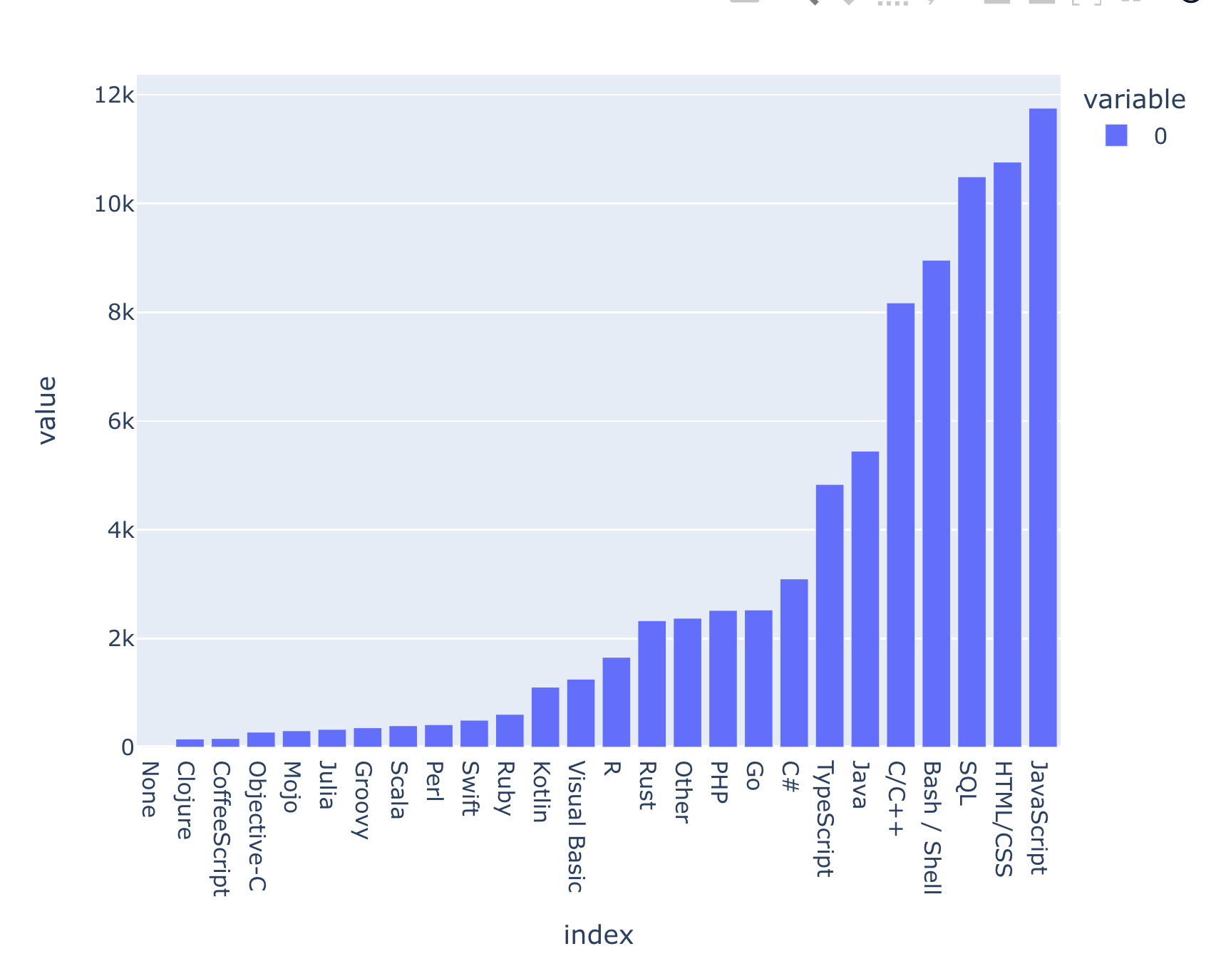
We can see that far and away, Python people are also using JavaScript, followed closely by HTML/CSS and SQL. Rust, which is gaining a lot of currency in the Python world, is still behind Java, TypeScript, and C#, but is more popular than a number of other languages that I've heard of and used, such as R, Ruby, and Perl. (And indeed, Perl is used more often than Scala and Julia? Wow.)