


This week, we looked at electric vehicle (EV) sales in the United States. I've always been struck by the small number of EVs on the road in the US, as well as the small number of makes and models that I see while there – especially when you are used to seeing a huge proportion of EVs, from a dozen or more manufacturers, in Europe and Israel.
The budget that the Trump administration signed into law last week will likely lead to fewer EV sales in the US. That's because the US has offered tax credits and rebates for about two decades, in order to encourage people to buy such cars. These incentives were cancelled by the new law, and will end on September 30th (https://www.marketplace.org/story/2025/07/08/ev-tax-credits-will-end-september-30-after-nearly-20-years).
This led me to wonder: How many EVs have really been sold over the last few years? Has the US seen an uptick in the number of EVs sold? Where are these EVs being sold?
Data and six questions
This week's data comes from the US Department of Transportation's Bureau of Transportation Statistics. Their site, at https://www.bts.gov/browse-statistical-products-and-data/state-transportation-statistics/electric-vehicle-registrations , shows EV registrations, other vehicle registrations, and EVs' electrical consumption. It includes data for the entire United States, and then per-state data, as well.
Sadly, data from 2024 only includes the total EV consumption, and not vehicle registrations. We'll thus have to make do with registration data from 2023 and earlier.
You can download the data file by clicking on the download button at the bottom of the displayed table; it looks like a rectangle with an arrow pointing down, and will show, "Choose a format to download" in the tooltip when you hover over it. Click on the icon, and choose "crosstab" as the data format you want, then choose "Excel." This will download an Excel document ("Sheet 1.xlsx") onto your computer.
Paid subscribers, including members of my LernerPython+data platform, can download the data file from the end of this message. You'll also find a copy of the Jupyter notebook I used to solve these problems, and a one-click link to open it in Google Colab.
I've also recorded a YouTube video of me solving the first two questions:
That's part of my Bamboo Weekly playlist, which you can view here: https://www.youtube.com/watch?v=wf_nbP-S5rk&list=PLbFHh-ZjYFwG34oZY24fSvFtOZT6OdIFm
This week's learning goals include: Working with Excel files, multi-indexes, window functions, and plotting with Seaborn.
Meanwhile, here are my six questions:
Read the Excel file into a Pandas data frame, using the first and second columns ("State" and the measurement category) as the two parts of a multi-index.
Let's start by loading Pandas:
import pandas as pdNext, we can use read_excel to load the file into a data frame:
filename = '/Users/reuven/Downloads/Sheet 1.xlsx'
df = pd.read_excel(filename)
The good news is that the file loads into a data frame just fine. However, we wanted the first two columns to be used in a multi-index.
We could invoke set_index to take any column (or columns) in a data frame and set them to be an index. That method returns a new data frame, which we can then assign back to the original variable.
But it's usually easier and faster to pass the index_col keyword argument to read_excel (or to read_csv, or any of a number of read_* methods in Pandas). Given that the first line of the file provides us with column names, we should thus be able to set the index using the State column and the second one.
But ... what is the second column's name? How can we access it? It doesn't have any text on the first row, whereas the other columns do.
When we read the Excel file into Pandas, we see that by default, Pandas assigns it a name of Unnamed: 1. Not only does that not give us a truly useful name, but it turns out that this name is given after index_col runs.
This code thus gave me an error:
df = pd.read_excel(filename,
                  index_col=['State', 'Unnmamed: 1'])
I solved the problem by using the numeric index of these columns, rather than their names. Remember that the column indexes start at 0, which means that I wrote:
df = pd.read_excel(filename,
                  index_col=[0, 1])
Sure enough, this defined df as a data frame with a two-part multi-index, with 364 rows and 9 columns. All of the columns were set to be int64 or float64, meaning that we're only dealing with numeric values (including NaN).
Excel files can contain more than one "sheet," and we can specify which one we want with the sheet_name keyword argument. In this case, however, there was only one sheet, so there was no need to specify it.
Using Seaborn, create a line plot showing the proportion of EV registrations in each year for which we have data (i.e., 2016 - 2023) over the entire US. Do we see an obvious trend?
To get data for the entire United States, and for the years, 2016 - 2023, we'll start with loc. Remember that we can invoke loc either with a single argument (a row selector) or with two arguments (a row selector and a column selector).
To get just a row, we can say:
(
    df
    .loc['United States']
)
Notice that because we have a two-level multi-index, we're able to choose the rows via the outer index ('United States'). The result is a data frame with all of the columns from the original, and only those rows for the entire United States. The index of this smaller, returned data frame is the inner part of the two-part multi-index.
We don't want data from 2024, because there isn't any. So maybe we can use range to specify the columns we want, and retrieve them that way:
(
    df
    .loc['United States', range(2018,2024)]
)
Unfortunately, this result in an error:
KeyError: "None of [Index([2018, 2019, 2020, 2021, 2022, 2023], dtype='int64')] are in the [columns]"How can that be? Because while the column names look like integers, they aren't – they are actually strings. In theory, we could convert them to strings, perhaps using a list comprehension. But in practice, we really only want to drop the 2024 column. We can do that with the drop method, specifying that we want to drop a column, not a row:
(
    df
    .loc['United States']
    .drop(columns=['2024'])
)
In order to find out the proportion of EVs, we'll only need two rows – the EV registrations row and the Total Vehicle Registrations row. We can retrieve those with loc, passing a list of indexes inside of the []:
import seaborn as sns

(
    df
    .loc['United States']
    .drop(columns=['2024'])
    .loc[['EV registrations', 'Total Vehicle Registrations']]
)
Next, I want to calculate the proportion of EVs in the US. To do that, I'll want to divide the top row (EV registrations) by the bottom row (Total Vehicle Registrations). There are a few ways I could do that, but I decided that it would be easier to invoke transpose (via its alias T), and flipping the rows and columns.
That made it easier and more natural to divide the EV registrations into the Total Vehicle Registrations, using a combination of assign and a lambda function. The result was a new column, ev_pct, showing the percentage of EVs in each year:
import seaborn as sns

(
    df
    .loc['United States']
    .drop(columns=['2024'])
    .loc[['EV registrations', 'Total Vehicle Registrations']]
    .T
    .assign(ev_pct = lambda df_: df_['EV registrations'] /
               df_['Total Vehicle Registrations'] * 100)
)
I used [] to retrieve just that column.
But then I wanted to plot it using Seaborn. (Why? Because I hadn't used Seaborn in a while here in Bamboo Weekly, and thought it would help to mix things up a bit. Besides, it's a fantastic plotting library and works very well with Pandas data frames.)
The thing is, Seaborn's functions aren't Pandas methods. So yes, I could invoke sns.lineplot and pass it my data frame. But if I want to use a method chain, I'm in a bit of trouble.
The solution is the pipe method, which allows us to take a function whose first argument is a series, and effectively invoke it as a method.
The way we do this is:
- We
import seaborn as sns, to have access to the Seaborn module - We invoke
.pipeon the['ev_pct']series we created - We pass
pipealambdafunction, that takes our series as an argument - We invoke
sns.lineplot, passing the series index as thexaxis and the series values on theyaxis:
import seaborn as sns


(
    df
    .loc['United States']
    .drop(columns=['2024'])
    .loc[['EV registrations', 'Total Vehicle Registrations']]
    .T
    .assign(ev_pct = lambda df_: df_['EV registrations'] /
               df_['Total Vehicle Registrations'] * 100)
    ['ev_pct']
    .pipe(lambda s_: sns.lineplot(x=s_.index,
                                      y=s_.values))
)
The result:
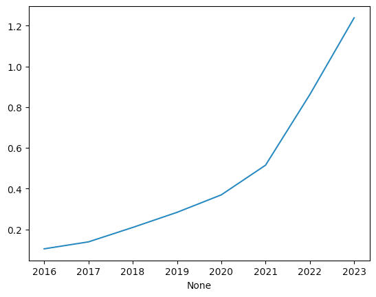
We can see a definitely upward spike in the popularity of EVs over the last number of years, and that number has accelerated in just the last 2-3 years.
However, look at the scale on the left – even after this rapid increase, the US is still at just over 1.2 percent EVs.