


This week, we looked at data from the most recent "Manufacturing Business Outlook Survey" conducted by the Philadelphia Federal Reserve (https://www.philadelphiafed.org/surveys-and-data/regional-economic-analysis/manufacturing-business-outlook-survey) since May 1968. This survey, often called the "Philadelphia Fed survey," asks manufacturers how things are going now, and what they think about the future. The most recent survey came out last week (https://www.philadelphiafed.org/surveys-and-data/regional-economic-analysis/mbos-2025-04), and indicates that many businesses are concerned.
Data and five questions
You can download the data for the survey from the survey's data page at
https://www.philadelphiafed.org/surveys-and-data/mbos-historical-data
I downloaded the complete history file in CSV format from:
The data dictionary will be a crucial part of understanding what columns to retrieve and process; you can find it here:
https://www.philadelphiafed.org/-/media/FRBP/Assets/Surveys-And-Data/MBOS/Readme.txt
This week's learning goals include working with dates and times, plotting, and filtering.
If you're a paid subscriber, then you'll be able to download the data directly from a link at the bottom of this post (although you should really use the API), download my Jupyter notebook, and click on a single link that loads the notebook and the data into Google Colab.
Also: A video walk-through of me answering this week's first two questions is on YouTube at https://youtu.be/2ike8xQsZAI. Check out the entire Bamboo Weekly playlist at https://www.youtube.com/playlist?list=PLbFHh-ZjYFwG34oZY24fSvFtOZT6OdIFm !
Here are my five questions:
Read the CSV data into a Pandas data frame. Make the DATE column into the index, as a datetime value.
We'll start, as usual, by loading up Pandas:
import pandas as pd
Next, I want to load the CSV file into a Pandas data frame. I can do that with read_csv:
filename = 'data/bw-116-bos_history.csv'
df = pd.read_csv(filename)
This works, in no small part because the first row of the file contains column names, and the values (except for the first column) are all floating-point numbers.
But that first column, whose name is DATE, contains date values – specifically, it contains month names and two-digit years, as in "Apr-25". I asked you to load that column as datetime values; as things currently stand, they're treated as strings.
Normally, read_csv doesn't try to parse dates and times; if it can identify a column as integers, it gives a dtype of int64, if it can identify it as containing floats, then it gives a dtype of float64, and in all other cases, it creates Python strings, referring to them as dtype of object.
We can force read_csv to parse a column as a datetime value by passing the parse_dates keyword argument, giving it a list of column names (or index numbers, if you prefer) that should be parsed as dates. We can thus say:
filename = 'data/bw-116-bos_history.csv'
df = pd.read_csv(filename,
                parse_dates=['DATE']
                )
Except that this won't work, because parse_dates can only handle a handful of unambiguous, well-known date formats. In order to parse this special format, we'll need to pass the date_format keyword argument, giving it a string that describes what we have here – namely, a three-letter month abbreviation (%b), a minus sign, and a two-digit year (%y). The date format codes have been standard in Python (and other languages) for many years, documented at https://docs.python.org/3/library/datetime.html#strftime-strptime-behavior .
A more modern, and better, way to parse and format dates is the amazing https://www.strfti.me/ site, which lets you experiment with formats and also gives you hints as to the formatting.
I can successfully read DATE into a data frame with datetime values with:
filename = 'data/bw-116-bos_history.csv'
df = pd.read_csv(filename,
                parse_dates=['DATE'],
                date_format='%b-%y')
This is fine, except for one small thing, namely that I asked you to turn the DATE column into the data frame's index. We could do that by taking the resulting data frame and invoking set_index on it, but why work so hard? We can pass the index_col keyword argument to read_csv, and it'll all be done at once:
filename = 'data/bw-116-bos_history.csv'
df = pd.read_csv(filename,
                parse_dates=['DATE'],
                date_format='%b-%y',
                index_col='DATE')
The result is a data frame with 684 rows and 168 columns. The index contains datetime values, and the rest are all float64.
Reproduce the plot at https://www.philadelphiafed.org/surveys-and-data/regional-economic-analysis/mbos-2025-04, showing the diffusion index for current and future general activity, both seasonally adjusted. By how much did the current seasonally adjusted diffusion index for general activity drop since the last survey?
The summary of the April survey included a graph that showed the seasonally adjusted diffusion index for general activity. I was wondering if you could recreate that. Plotting this data sounds like the easy part; from where do we retrieve it?
The data dictionary (https://www.philadelphiafed.org/-/media/FRBP/Assets/Surveys-And-Data/MBOS/Readme.txt) is often the most important part of any data set. Every data set uses different codes and abbreviations, and has its own idiosyncrasies. This data dictionary was particularly unusual; once you get the hang of it, then you can understand how they laid it out, but it took me a while.
Basically, every column has six or seven characters:
- The first two characters represent the type of data that was retrieved. So "ga" is "general activity," and "pp" is "prices paid."
- The next character, which the data dictionary represents with
$, is either "c" (for "current") or "f" (for "future"). The survey asked manufacturers whether (for example) general activity is currently increasing, decreasing, or remaining the same, and also whether they expect, six months in the future, for general activity to be increasing, decreasing, or remaining the same. - Next, we might have two characters, "df", meaning the "diffusion index," calculated by subtracting the "decreasing" number from the "increasing" number. We might also have one character, for those columns representing the raw data, in columns named with "d" ("decreasing"), "n" ("no change"), or "i" ("increasing"). So you can grab the raw data, or you can just look at the pre-calculated diffusion index for each metric.
- Next, the data dictionary contains
#, which can be either "s" (for seasonally adjusted data) for "n" (for non-seasonally adjusted data). - Every column name then ends with "a", which I'm guessing means "aggregation," but I am not sure.
So, for the plot, we'll want:
- "ga" for general activity
- "c" for current activity and "f" for future activity
- "df" for the diffusion index
- "s" for seasonally adjusted
- "a"
We can retrieve those two columns as:
(
    df
    [['gacdfsa', 'gafdfsa']]
)
But if we take a close look at the plot that the Philadelphia Fed provided, we see it only starts in 2011. Fortunately, because our data frame's index contains datetime values, we can use loc and specify the years we want. Here, we'll just use a slice, starting in 2011 and going to the end:
(
    df
    .loc['2011':]
    [['gacdfsa', 'gafdfsa']]
)
We can then create a line plot with this data by invoking plot.line:
(
    df
    .loc['2011':]
    [['gacdfsa', 'gafdfsa']]
    .plot.line()
)
And we get:
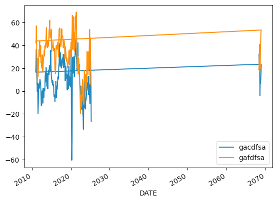
Um... something seems to have gone wrong here. The data does start in 2011, but it ends in 2070? I know that the Philadelphia Fed survey is supposed to include companies' forecasts for the future, but this seems a bit extreme, no?
The problem, of course, stems from how we read the data into Pandas: Because the data contains only two-digit years, the system needs to decide whether "20" is "1920" or "2020". It turns out that "Jan-69" is seen as January, 1969, as we would want and expect. But "Dec-68" is seen as December 2068! We can see that here, invoking pd.to_datetime:
pd.to_datetime(['Dec-68', 'Jan-69'], format='%b-%y')The result:
DatetimeIndex(['2068-12-01', '1969-01-01'], dtype='datetime64[ns]', freq=None)I'm willing to ignore the data from 1968, but that means we'll need to cap our loc in the current year (2025), just to be sure that we aren't getting weird data from the pseudo-future. In order to do that, we'll need to first invoke sort_index, since the slice on years won't work if the years are out of order, and the 2068 dates (!) are currently at the top of the data frame:
(
    df
    .sort_index()
    .loc['2011':'2025']
    [['gacdfsa', 'gafdfsa']]
    .plot.line(ylim=(-80, 80), grid=True)
)
Finally, in order to make the grid match the one that we saw in the Philadelphia Fed report, I passed the ylim keyword argument to plot.line, giving a tuple of minimum and maximum y values. I also asked for grid=True, so that we would have a light grid in the background:
(
    df
    .sort_index()
    .loc['2011':'2025']
    [['gacdfsa', 'gafdfsa']]
    .plot.line(ylim=(-80, 80), grid=True)
)
The results:
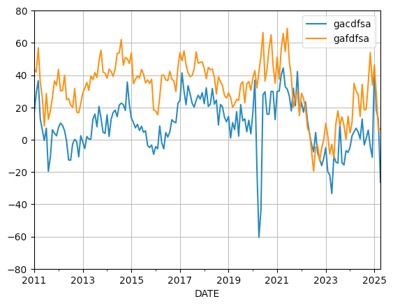
We can see, over on the right side of the graph, that both of the lines (for both current and future values) have declined quite a bit. I asked you to find out by how much; we can find out by invoking diff (to get the absolute difference between rows) and pct_change (to get the percentage difference between rows). To get both of these, I use the agg method, which lets me get more than one aggregation value:
(
    df
    ['gacdfsa']
    .agg(['diff', 'pct_change'])
    .iloc[-1]
)
Notice that I'm only interested in the most recent change, so I grab iloc[-1], and get:
diff         -38.900
pct_change    -3.112
Name: 2025-04-01 00:00:00, dtype: float64
In other words, the absolute number declined by 39 points in the last month, a change of -3 percent. And sure enough, in their report, the Philadelphia Fed writes, "he diffusion index for current general activity dropped 39 points to -26.4 in April, its lowest reading since April 2023 (see Chart 1)." So yes, we managed to recreate it!