


This week’s topic: Bank failures
This week, we looked at describing bank failures and assistance, which I (perhaps unfairly!) lumped into a single category of “failures.” This, of course, comes in the wake of the collapse of Silicon Valley Bank.
Our data set comes from the FDIC itself. You can download it in CSV format from:
https://banks.data.fdic.gov/explore/failures?aggReport=detail&displayFields=NAME%2CCERT%2CFIN%2CCITYST%2CFAILDATE%2CSAVR%2CRESTYPE%2CCOST%2CRESTYPE1%2CCHCLASS1%2CQBFDEP%2CQBFASSET&endFailYear=2023&sortField=FAILDATE&sortOrder=desc&startFailYear=1934Our questions for this week are:
- According to our document, how many bank failures have there been since the FDIC was opened?
- What was the earliest failure in our data set? What is the most recent failure in our data set?
- In which five years did the greatest number of banks fail?
- In which three states were the greatest number of failed banks?
- What was the average market capitalization of the banks that failed? Given a capitalization of $200b, did that make SVB above, below, or about average?
- When was the most recent failure greater than SVB?
- Bank failures can be resolved in several different ways. How often, historically, have we seen each resolution? Were the odds good that SVB's uninsured depositors would get their money?
- What about bank failures in the last 25 years -- if we just look at those, do the odds change?
- What was the mean estimated loss in bank failures? What proportion of a bank's assets did this generally involve?
The learning goals for this week include working with dates and strings. And some insights into whether people were right to panic about losing their money when SVB went under.
Discussion
First, before anything else, I did my standard setup for working with Pandas:
import numpy as np
import pandas as pd
from pandas import Series, DataFrame
Then I had to retrieve the file and turn it into a data frame. Getting the URL accurate took a bit of time; it was only as I was doing the calculations that I discovered the default download starts in 2012, long after the FDIC started!
The URL is thus
https://banks.data.fdic.gov/explore/failures?aggReport=detail&displayFields=NAME%2CCERT%2CFIN%2CCITYST%2CFAILDATE%2CSAVR%2CRESTYPE%2CCOST%2CRESTYPE1%2CCHCLASS1%2CQBFDEP%2CQBFASSET&endFailYear=2023&sortField=FAILDATE&sortOrder=desc&startFailYear=1934That URL takes us to a page from which we can download the data.
In my code, I handled it as follows, with read_csv, passing it a URL (rather than a downloaded filename):
data_url = 'https://pfabankapi.app.cloud.gov/api/failures?fields=NAME%2CCERT%2CFIN%2CCITYST%2CFAILDATE%2CSAVR%2CRESTYPE%2CCOST%2CRESTYPE1%2CCHCLASS1%2CQBFDEP%2CQBFASSET&filters=FAILYR%3A%5B1934%20TO%202023%5D&limit=10000&react=true&sort_by=FAILDATE&sort_order=desc&subtotal_by=RESTYPE&total_fields=QBFDEP%2CQBFASSET%2CCOST&format=csv&download=true&filename=bank-data'

df = pd.read_csv(data_url)
That loaded the data frame just fine. However, it wasn’t quite good enough for our purposes. That’s because the “FAILDATE” column contains date information, and we’ll need the date for our calculations. We can force Pandas to treat FAILDATE as a datetime column by passing the parse_dates keyword argument:
df = pd.read_csv(data_url,
                parse_dates=['FAILDATE'])
We won’t be needing all columns of the data frame, but it’s a small enough data set that I’m OK keeping them around, without any more filtering.
And with that, let’s move onto the first question!
According to our document, how many bank failures have there been since the FDIC was opened?
Assuming that each row in the data frame represents one bank failure, we merely need to grab the “shape” attribute from our data frame:
df.shape(Remember that shape is an attribute, not a method! Trying to invoke it will result in an error.)
Of course, that returns a 2-element tuple with the number of rows and the number of columns. So you would have to retrieve index 0 from the resulting tuple to just get the number of rows.
Another way to get the number of rows is with:
len(df.index)I’ve heard that this is the best, most idiomatic way to do it, in part because the index is a known length, and that it runs fastest. I know myself, though, and I tend to just get the shape, and look at the first element of the returned tuple.
What you should not do is invoke the “count” method, because it ignores NaN values. Plus, it’ll return a series indicating the number of non-NaN values in each column of the data frame.
What was the earliest failure in our data set? What is the most recent failure in our data set?
To get the earliest failure, we need to sort by “FAILDATE”, the column which we made sure to import as a date in our call to “read_csv”.
Remember that datetime objects are comparable, which means that we can use operators such as < and > on them. This also means that we can sort them. But while we could invoke sort_values on our data frame, then grabbing the first (or last) element, here we’re only interested in the date.
As such, it’s probably easiest to just call “min” and “max” on that column. The minimum is:
df['FAILDATE'].min()returning April 19th, 1934, and the maximum is
df['FAILDATE'].max()returning October 23rd, 2020. So none of the latest failures have made it into the database as of yet. It’s almost as if the FDIC had something else to do right now.
What if we want to get both the min and max at the same time? The “agg” method lets us specify any aggregation function, or even a list of such functions:
df['FAILDATE'].agg(['min', 'max'])In which five years did the greatest number of banks fail?
Once again, we’ll turn to “FAILDATE”, this time to extract the year in which the bank failed. Because we have a datetime object, we can use the “dt” accessor to retrieve any of its constituent parts. In this case, we can get the year from each record with “.dt.year”:
df['FAILDATE'].dt.yearGiven the series of years that was returned, we can then invoke “value_counts”, and find out how often each year appears in our data set:
df['FAILDATE'].dt.year.value_counts()Because value_counts automatically sorts the data from most to least common, we can invoke “head(5)”, and see only the five years that most often appear in our data set:
df['FAILDATE'].dt.year.value_counts().head(5)To be honest, I was a bit surprised that we saw most of the numbers in the late 1980s and early 1990s:
1989    534
1988    470
1990    382
1991    271
1987    262
But then I remembered the savings and loan crisis from that time. I had completely forgotten how many banks (or S&Ls) went out of business at the time.
In which three states were the greatest number of failed banks?
I was curious to know if there were particular states where more banks had failed. This might not be a particularly fair comparison, given that some states are larger than others, and some have specifically tried to attract banks to set up shop. But still it might be interesting to see.
The data frame does have geographical information about each failed bank, in the “CITYST” column. However, as the name implies, this column contains both the city and the state. In order to perform our analysis, we’ll need to retrieve just the state.
To do that, we’ll need to understand what the data looks like. Here are the first five values of CITYST:
0               ALMENA, KS
1    FORT WALTON BEACH, FL
2        BARBOURSVILLE, WV
3              ERICSON, NE
4               NEWARK, NJ
Name: CITYST, dtype: object
As you can see, the data here contains a city name, a comma, a space, and then a two-letter state abbreviation. If we can somehow grab that two-letter state from the end of the string, we’ll be in great shape.
If we were in regular Python, then we could use a slice to retrieve a substring by specifying the starting index and the ending index. For example, we could say
s = ‘abcdefg’
print(s[2:5])    # prints cde
In this case, it would print “cde”, because we asked for the slice starting at index 2 and ending before index 5.
What if we want from index 2 through the end of the string? We can say:
s = ‘abcdefg’
print(s[2:])     # prints cdefg
Notice how we leave off the endpoint, which tells Python to read through the end of the string.
What if we want the final two characters? We could, of course, specify the index in this example with 5. But if we don’t know the length of the string, it gets trickier. Luckily, Python provides us with a solution: We can use a negative index to read from the right side of the string. For example:
s = ‘abcdefg’
print(s[-2:])     # prints fg
Reading from the right side, s[-1] is “g”, and s[-2] is “f”. So if we ask for the slice from -2 through the end of the string, we get “fg”.
How can we use this kind of slice in Pandas? We obviously don’t want to use a “for” loop. Fortunately, the “str” accessor provides us with access to a large number of string methods, including once aptly called “slice”.
But wait — slice is a method! When we used the slice with square brackets, we passed it -2 and … nothing. How can we represent that with the “slice” method?
The answer: Pass -2 as the first argument, and None as the second argument. Indeed, under the hood in Python, when you say s[-2:], that’s really translated into a call to the builtin slice, passing it arguments (-2, None). We can thus say:
df['CITYST'].str.slice(-2, None)This returns a new series, in which each element is a two-character string, the abbreviation of a state. We want to know how many times each state appeared in this data set, and can do that with our old friend “value_counts”:
df['CITYST'].str.slice(-2, None).value_counts()Finally, we can find the three states that appeared most often in our data set
df['CITYST'].str.slice(-2, None).value_counts().head(3)I got the following results:
TX    910
CA    263
IL    227
Name: CITYST, dtype: int64
As you can see, Texas has had much larger number of bank failures over the years than any other state. I’m guessing that this has to do with the S&L crisis, given that so many of them were chartered in Texas.
Just for fun, I ran a query to find out when Texas banks failed:
df.loc[df['CITYST'].str.slice(-2, None) == 'TX', 'FAILDATE'].dt.year.value_counts().head(10)The numbers seemed pretty compelling:
1988    256
1989    224
1990    140
1987     68
1991     41
1992     31
1986     31
1985     17
1982     16
1993     10
Name: FAILDATE, dtype: int64
But it was even more obvious when I ran this code:
df.loc[df['CITYST'].str.slice(-2, None) == 'TX', 'FAILDATE'].dt.year.plot.hist()That returned a histogram with the “plot.hist” method:
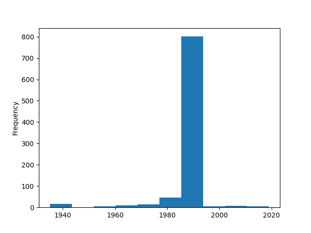
Yeah, I’d say that there was some sort of banking crisis in Texas in the late 1980s!
What was the average market capitalization of the banks that failed? Given a capitalization of $200b, did that make SVB above, below, or about average?
Here, I decided to count the proportion of banks whose capitalization was above $200b. I first ran a query against the QBFASSET column:
df['QBFASSET'] > 200_000_000This returns a boolean series. We can then count the number of True and False values:
(df['QBFASSET'] > 200_000_00
0).value_counts()
I got the following results:
False    4101
True        3
Name: QBFASSET, dtype: int64
So in the entire history of FDIC failures, only three banks were larger than Silicon Valley Bank. Wow. (Granted, if we were doing a serious analysis here, we would likely want to take inflation into account. But still.)
We can turn this into a percentage by passing the “normalize” keyword argument:
(df['QBFASSET'] > 200_000_000).value_counts(normalize=True)The result?
False    0.999269
True     0.000731
Name: QBFASSET, dtype: float64
In other words, SVB was bigger than 99.9% of the banks that have failed in the FDIC’s history.
When was the most recent failure greater than SVB?
Maybe SVB was an unusually large bank to fail, but we know that there were larger ones. The question is, when did that happen most recently?
To find that, we’ll first need to get all of the banks with capitalizations larger than $200b in our data set. We’ll first use our mask index from before, applying it to the entire data frame:
df.loc[df['QBFASSET'] > 200_000_000]This returns only those rows in “df” where the failed bank’s market cap was greater than $200b. We can sort the resulting data frame by the FAILDATE column, in descending order:
df.loc[df['QBFASSET'] > 200_000_000].sort_values('FAILDATE', ascending=False)Finally, we can look at the first element in that sorted data frame:
df.loc[df['QBFASSET'] > 200_000_000].sort_values('FAILDATE', ascending=False).head(1)The result? Bank of America, based in Charlotte, North Carolina, which failed in 2009.
I reacted to this with a bit of surprise. After all, I’m far from an expert in US banks, but Bank of America still exists, no? What’s going on?
I’m not completely sure, but it looks like, as part of the great recession and banking crisis that started in 2008, Bank of America got some help from the US government, got back on its feet, and then repaid the government.
https://www.federalreserve.gov/newsevents/reform_boa.htm
I could definitely be wrong about this, but that’s my best reading as a non-expert.
Bank failures can be resolved in several different ways. How often, historically, have we seen each resolution? Were the odds good that SVB's uninsured depositors would get their money?
Let’s say a bank fails. What happens then?
In the bad old days, the bank would close, and the depositors would lose their money. The whole point of the FDIC is to give people some peace of mind, to know that their money is safe, and that they don’t need to start checking out their bank’s reliability before becoming a customer.
But the FDIC has several different options at its disposal. They can have another bank come in, buy the assets of the failed bank, and take it over. From the customers’ perspective, it’s as if their bank had been bought by another bank. (Because that’s basically what it is.) The buying bank makes a deal with the government, such that they don’t have to pay very much — for example, the UK branch of Silicon Valley Bank was acquired by a big UK bank, HSBC, for the price of £1. And if you’re thinking, “Hmm, maybe I could buy a bank for that price,” remember that they also took on the customers and liabilities.
Another option is for the bank to go out of business completely, for the FDIC to give customers any money they had, up to $250k. Any account with more than that is wiped out.
That’s the scenario that people were worried about with SVB. The crypto company Circle apparently had $3b in their SVB account; $250k really wouldn’t have done much for them. (Insert your own cryptocurrency joke here, please.)
As it turns out, the US government announced that all account holders would get their money, not just those with up to $250k. How often does this happen? How often does everyone get their money back?
Fortunately, the FDIC can tell us. The “RESTYPE” column tells us whether the bank needed assistance, or if it failed. I’m again going to stress that while these are different scenarios, we’re going to treat all of the data as a failure, to make it easier on ourselves. We’ll thus look at the oh-so-cleverly named “RESTYPE1” column, and run “value_counts” on it, to see the different possibilities. I throw in normalize=True to see the percentages:
df['RESTYPE1'].value_counts(normalize=True)What do we see?
PA      0.510965
A/A     0.141082
PO      0.139620
IDT     0.094055
P&A     0.061160
PI      0.034113
MGR     0.009016
ABT     0.003899
OBAM    0.003168
DINB    0.002193
REP     0.000731
Name: RESTYPE1, dtype: float64
Now, I’m no banker, but the data dictionary and explanation at the FDIC’s site can tell us what all of these are. Here are explanations of the top few:
- PA: Purchase and assumption, where another bank takes over for the existing institution. Everyone, insured and uninsured, gets their money.
- A/A: Assistance transactions, where the bank survives (in other words, doesn’t fail), and the government helps to keep them going.
- PO: The bank fails completely, and the FDIC pays people up to $250k
- IDT: Insured deposit transfer; to the best of my understanding, insured depositors definitely get their money (i.e., up to $250k) and everyone else gets something, but not necessarily everything, from the acquiring institution
- P&A: Yes, this is different from PA! Another bank buys the assets of the failed bank, and it’s not clear if all of the assets were purchased, or just the insured ones.
- PI: Another bank buys the failed bank’s insured deposits. The uninsured ones go away.
The top two options (PA and A/A) account for 65 percent of bank failures in the entire history of the FDIC. In those cases, no one lost money, even if they had beyond the insured amount of $250k. So we had good reason to hope that SVB’s customers would all be bailed out.
What about bank failures in the last 25 years — if we just look at those, do the odds change?
The FDIC has been around for a long time, and both banks and bank regulations have changed a lot. Maybe if we just look at the most recent 25 years, we’ll see that things are better, or worse?
To do that, I first ran a query to find all bank failures since January 1st, 1998:
df['FAILDATE'] > '1998-01-01'I got back a boolean series, and applied that as a mask index to our data frame. I’m only interested in the “RESTYPE1” column, so I specified that as the second argument to .loc:
df.loc[df['FAILDATE'] > '1998-01-01', 'RESTYPE1']This gave me the resolutions for bank failures in the last 25 years. I could then run value_counts with normalize=True:
df.loc[df['FAILDATE'] > '1998-01-01', 'RESTYPE1'].value_counts(normalize=True)The results?
PA      0.864865
PI      0.060811
PO      0.038851
OBAM    0.021959
DINB    0.013514
Name: RESTYPE1, dtype: float64
Wow! In 86 percent of the cases from the last 25 years, even when banks went out of business, they were acquired by someone and everyone — insured and uninsured — depositors got to keep their money.
So while the US government’s announcements about helping SVB and making sure everyone got to keep their money were welcome news, they’re not that surprising, given the history.
What was the mean estimated loss in bank failures? What proportion of a bank's assets did this generally involve?
Finally, a bank failure does cost something. How much did it typically cost? We can find out by looking at the COST column:
df['COST'].mean()We see that it cost, on average, $74m to bail out a bank.
Fine, but if we compare that with a bank’s assets, how much did it cost? Here, we’ll just divide the cost into the bank’s capitalization:
(df['COST'] / df['QBFASSET']).mean()On average, about 25% of the capitalization was lost. Truth be told, that number seems a bit fishy to me; I can’t imagine that it’ll cost $50b to bail out SVB! So maybe I’m not understanding things here? Or maybe, it differs by resolution type.
I’m going to create a new column, COST_PER, which calculates the cost per failure:
df['COST_PER'] = df['COST'] / df['QBFASSET']Then I’ll find out, per resolution type, how much it cost, on average:
df.groupby('RESTYPE1')['COST_PER'].mean()Even in the best-case scenario, PA, it looks like the bank loses about 21 percent of its assets. But again, I’m sure I’m misreading something here, and would be happy to get insights from you in the comment thread.
That’s it for this week. I’ll be back next Wednesday with more data and the news. Please let me know what you think; Bamboo Weekly is still new, and I’m trying to figure out how to improve it. And of course, if you have suggestions for topics, data sets, and Pandas features to explore, let me know!
Meanwhile, here’s my notebook for this week: https://drive.google.com/file/d/1II5svSQFA2iTM1MzZuZOA0xJ8SAnii5M/view?usp=drive_link
Reuven