


This week, we looked at electric cars — where people are (and aren’t) buying them, and how much the picture has changed in the last few years.
This topic was inspired by a combination of current events — specifically, the Biden Administration’s plans to levy massive tariffs on Chinese-made electric cars (https://www.nytimes.com/2024/05/15/business/economy/china-electric-vehicles-biden-tariffs.html?unlocked_article_code=1.t00.LpnP.Iciy7ilqMVES&smid=url-share), along with my surprise at seeing so few electric cars on American roads, when compared with my experience in Israel, Iceland, and Europe.
Data and six questions
This week's data comes from the most recent “Global EV outlook” released last month by the International Energy Agency (IEA), available at https://www.iea.org/reports/global-ev-outlook-2024. The data is downloadable from their "data explorer" page:
https://www.iea.org/data-and-statistics/data-tools/global-ev-data-explorer
You can download the data, or parts of it, by going to the above URL and selecting "ev sales," "cars," and "world" on the pull-down menus. Then click on "download data," and the CSV file should be downloaded to you.
Here are my six tasks and questions for this week. They have to do with filtering, grouping, multi-indexes, pivoting, piping, and also styling Pandas data frames. As always, I'll be back tomorrow with my full solutions, including the Jupyter notebook I used in my solution:
Read the EV data into a data frame. Remove rows from the "world" region. Keep only those rows with "EV sales" and "EV stock" parameters.
Let’s start, as usual, by loading Pandas:
import pandas as pdWith that in place, we can then load the CSV file into a data frame, using “read_csv”:
filename = 'IEA-EV-dataEV stock shareHistoricalCars.csv'


df = (
    pd
    .read_csv(filename)
)
However, we only want to keep those rows in which the “parameter” column has a value of either “EV sales” or “EV stock”. I’ll use “.loc” to retrieve those rows that match this description by passing it a “lambda” expression, one that gets a data frame as an argument. I’ll use a parameter name of “df_” to indicate that it’s a local variable temporarily assigned a data frame.
But what should our “lambda” expression do? Return a boolean series, indicating where the row contains the value “EV sales” or “EV stock”. There are a few ways we can do that, but the “isin” method, passed a list of strings, is my favorite way to do this:
df = (
    pd
    .read_csv(filename)
    .loc[lambda df_: df_['parameter'].isin(['EV sales', 'EV stock'])]
)
The resulting data frame now only has “EV sales” and “EV stock” rows. However, I also asked you to remove rows in which the “region” column contains the value “World”. We can use a similar “lambda” expression there:
df = (
    pd
    .read_csv(filename)
    .loc[lambda df_: df_['parameter'].isin(['EV sales', 'EV stock'])]
    .loc[lambda df_: df_['region'] != 'World']
)
The resulting data frame, which we have assigned to “df”, now contains regions that aren’t “World” and with only EV sales and EV stock info.
Create a data frame showing the number of cars sold each year, in each country, with a BEV ("battery electric vehicle") powertrain.
To create such a data frame, we’ll need to take our existing “df” and then cut it down a bit. First, we’ll keep only those rows in which the “parameters” column contains the value “EV sales”, again using “loc”:
(
    df
    .loc[lambda df_: df_['parameter'] == 'EV sales']
)
Next, we’ll keep only those rows in which the “powertrain” column contains the value “BEV”, for “battery electric vehicle:
(
    df
    .loc[lambda df_: df_['parameter'] == 'EV sales']
    .loc[lambda df_: df_['powertrain'] == 'BEV']
)
But now we need to pull out the big guns. We want to get a new data frame in which:
- The index contains the years, the distinct values from the “year” column
- The column names are the distinct values from the “region” column
- The values are taken from the “value” column
To do this, we can create a pivot table on “df”, using the “pivot_table” method:
(
    df
    .loc[lambda df_: df_['parameter'] == 'EV sales']
    .loc[lambda df_: df_['powertrain'] == 'BEV']
    .pivot_table(index='year',
                columns='region',
                values='value')
)
The result is a rejiggering of our data, letting us see just how many EVs were sold in each country over the last number of years.
In many cases, the differences are staggering — such as 4 (yes, four) vehicles in Sweden in 2010, and 110,000 in 2013. Or 1,100 vehicles in China in 2010, versus 5,400,000 in 2013.
In which five countries have we seen the greatest percentage growth in the number of EV cars sold between 2019 and 2023?
In order to answer this question, we’ll need to start with the pivot table from the previous question:
(
    df
    .loc[lambda df_: df_['parameter'] == 'EV sales']
    .loc[lambda df_: df_['powertrain'] == 'BEV']
    .pivot_table(index='year',
                columns='region',
                values='value')
)
With this in place, we can now calculate the percentage change (with “pct_change”) in each column, from one row to the next. However, we don’t want to know the percentage change from 2019 to 2020, 2020 to 2021, 2021 to 2022, etc.
We want to know the percentage change from 2019 to 2024. That’s a four-year gap, so we pass the “periods=4” keyword argument to “pct_change”, ensuring that it calculates what we want. We also pass “fill_method=None” to stop Pandas from warning us that the previous default value for handling missing values will soon be deprecated:
(
    df
    .loc[lambda df_: df_['parameter'] == 'EV sales']
    .loc[lambda df_: df_['powertrain'] == 'BEV']
    .pivot_table(index='year',
                columns='region',
                values='value')
     .pct_change(periods=4, fill_method=None)
)
We can then use “loc” to select only the row for the year 2023, which now contains the percentage difference from 2019 to 2023:
(
    df
    .loc[lambda df_: df_['parameter'] == 'EV sales']
    .loc[lambda df_: df_['powertrain'] == 'BEV']
    .pivot_table(index='year',
                columns='region',
                values='value')
    .pct_change(periods=4, fill_method=None)
    .loc[2023]
)
Finally, we can use “nlargest” to retrieve the five highest percentages:
(
    df
    .loc[lambda df_: df_['parameter'] == 'EV sales']
    .loc[lambda df_: df_['powertrain'] == 'BEV']
    .pivot_table(index='year',
                columns='region',
                values='value')
    .pct_change(periods=4, fill_method=None)
    .loc[2023]
    .nlargest(5)

)
We can see the results:
region
United Arab Emirates    695.969697
Turkiye                 285.956522
India                   119.588235
Israel                   56.647059
Mexico                   43.827586
Name: 2023, dtype: float64
I never would have guessed that of all countries, the UAE would have the greatest percentage growth in EV sales in over the last five years. But it would seem that’s the case!
Compare, for each year, the "stock" value with the "sales" value for cars with BEV powertrains. How much of the stock was sold, in each year, for each country? In what countries + years were sales equal to the stock? In what countries + years were sales less than 10% of the stock? Did such a low proportion of sales happen in 2022 or 2023?
So far, we have only looked at EV sales. But our data frame also contains information about EV stocks, meaning how many are on hand. I asked you to compare the number of sales with the number of EVs in stock.
We’ll again start with our pivot table:
(
    df
    .loc[lambda df_: df_['parameter'].isin(['EV sales', 'EV stock'])]
    .loc[lambda df_: df_['powertrain'] == 'BEV']
    .pivot_table(index=['region', 'year'],
                columns='parameter',
                values='value')
)
If I want, I can now divide EV sales by EV stock by saying
df['EV sales'] / df['EV stock']But this is much harder to do in a method chain. After all, a method chain runs on the entire data frame. And yes, I could retrieve a single column with `[]`, but what then? How do I get the second column?
What I’d like to do is write a function that takes a data frame as an argument, and then calls the function, passing “df” as the argument. I can’t do that with method chaining, though, can I?
Actually, you can: The “pipe” method exists for precisely this purpose, for invoking a function on the data frame as part of the method chain. Here, I’ll just write a “lambda” expression that performs the division described above:
(
    df
    .loc[lambda df_: df_['parameter'].isin(['EV sales', 'EV stock'])]
    .loc[lambda df_: df_['powertrain'] == 'BEV']
    .pivot_table(index=['region', 'year'],
                columns='parameter',
                values='value')
    .pipe(lambda df_: df_['EV sales'] / df_['EV stock'])
)
The result of invoking this function (via “pipe”) on our data frame is a series, on which we can then invoke “loc” and grab only those values equal to 1:
(
    df
    .loc[lambda df_: df_['parameter'].isin(['EV sales', 'EV stock'])]
    .loc[lambda df_: df_['powertrain'] == 'BEV']
    .pivot_table(index=['region', 'year'],
                columns='parameter',
                values='value')
    .pipe(lambda df_: df_['EV sales'] / df_['EV stock'])
    .loc[lambda s_: s_ == 1]
)
In which locations was the entire stock sold out?
region        year
Australia     2011    1.0
Brazil        2014    1.0
Chile         2011    1.0
Greece        2013    1.0
Korea         2010    1.0
              2018    1.0
Mexico        2011    1.0
South Africa  2013    1.0
Spain         2010    1.0
Sweden        2010    1.0
              2011    1.0
Switzerland   2011    1.0
dtype: float64
This hasn’t happened in a while, which I take to mean that companies are producing more EVs each year, and that they aren’t selling out — something that happened in the early days of EV sales.
Next, I asked you to find countries and years in which less than 10 percent of the EV stock was sold. This query is almost identical to the previous one, but looks for rows that are < 0.10, rather than == 1:
(
    df
    .loc[lambda df_: df_['parameter'].isin(['EV sales', 'EV stock'])]
    .loc[lambda df_: df_['powertrain'] == 'BEV']
    .pivot_table(index=['region', 'year'],
                columns='parameter',
                values='value')
    .pipe(lambda df_: df_['EV sales'] / df_['EV stock'])
    .loc[lambda s_: s_ < 0.10]
)
I can then invoke “unstack” to move the outer level of the multi-index (i.e., the region) to be the columns of a data frame:
(
    df
    .loc[lambda df_: df_['parameter'].isin(['EV sales', 'EV stock'])]
    .loc[lambda df_: df_['powertrain'] == 'BEV']
    .pivot_table(index=['region', 'year'],
                columns='parameter',
                values='value')
    .pipe(lambda df_: df_['EV sales'] / df_['EV stock'])
    .loc[lambda s_: s_ < 0.10]
    .unstack(level=0)
)
We get the following (formatted better on your screen, I hope):
region  Costa Rica   Denmark     India    Israel     Italy    Poland  Portugal
year
2015      0.028571       NaN       NaN  0.002500       NaN  0.028000       NaN
2016      0.075000       NaN       NaN  0.004167       NaN  0.042308       NaN
2017           NaN  0.080682       NaN  0.092857       NaN       NaN       NaN
2012           NaN       NaN  0.067857       NaN       NaN       NaN  0.056250
2019           NaN       NaN  0.079070       NaN       NaN       NaN       NaN
2011           NaN       NaN       NaN  0.035294       NaN       NaN       NaN
2014           NaN       NaN       NaN  0.005000       NaN       NaN       NaN
2018           NaN       NaN       NaN  0.086667       NaN       NaN       NaN
2010           NaN       NaN       NaN       NaN  0.061538       NaN  0.018056
Since neither 2022 nor 2023 are in the index, we can say that no, such low sales didn’t occur in any country in those years.
Which five countries, on average, have the highest percentage of sales / stock?
Now that we can calculate sales / stock, I asked you to find which five countries have the highest such mean values. We can again start with the pivot table on which we’ve run “pipe”:
(
    df
    .loc[lambda df_: df_['parameter'].isin(['EV sales', 'EV stock'])]
    .loc[lambda df_: df_['powertrain'] == 'BEV']
    .pivot_table(index=['region', 'year'],
                columns='parameter',
                values='value')
    .pipe(lambda df_: df_['EV sales'] / df_['EV stock'])
)
We’re now going to have to perform some grouping, and we’re going to use our two multi-index components when we do that. So I’ll move the index components to the data frame with “reset_index”, making them into regular columns.
We can then run a “groupby” operation, grouping on the “region” column, and performing “mean” on the values in column 0:
(
    df
    .loc[lambda df_: df_['parameter'].isin(['EV sales', 'EV stock'])]
    .loc[lambda df_: df_['powertrain'] == 'BEV']
    .pivot_table(index=['region', 'year'],
                columns='parameter',
                values='value')
    .pipe(lambda df_: df_['EV sales'] / df_['EV stock'])
    .reset_index()
    .groupby('region')[0].mean()
)
Here’s the result:
region
Australia               0.509556
Austria                 0.359467
Belgium                 0.511249
Brazil                  0.597556
Bulgaria                     NaN
Canada                  0.472746
Chile                   0.403045
China                   0.527578
Colombia                     NaN
Costa Rica              0.341232
Croatia                      NaN
Cyprus                       NaN
Czech Republic               NaN
Denmark                 0.372616
EU27                    0.413793
Estonia                      NaN
Europe                  0.395114
Finland                 0.391805
France                  0.436134
Germany                 0.515133
Greece                  0.524149
Hungary                      NaN
Iceland                 0.518910
India                   0.333311
Ireland                      NaN
Israel                  0.333586
Italy                   0.340381
Japan                   0.301969
Korea                   0.540066
Latvia                       NaN
Lithuania                    NaN
Luxembourg                   NaN
Mexico                  0.470482
Netherlands             0.441469
New Zealand             0.483830
Norway                  0.334612
Poland                  0.251607
Portugal                0.279091
Rest of the world       0.383455
Romania                      NaN
Seychelles                   NaN
Slovakia                     NaN
Slovenia                     NaN
South Africa            0.382541
Spain                   0.461403
Sweden                  0.547542
Switzerland             0.436222
Turkiye                 0.333446
USA                     0.384041
United Arab Emirates         NaN
United Kingdom          0.408701
Name: 0, dtype: float64
This is nice, but what are the countries with the highest sales ratio, on average? We’ll run “nlargest” on this data:
(
    df
    .loc[lambda df_: df_['parameter'].isin(['EV sales', 'EV stock'])]
    .loc[lambda df_: df_['powertrain'] == 'BEV']
    .pivot_table(index=['region', 'year'],
                columns='parameter',
                values='value')
    .pipe(lambda df_: df_['EV sales'] / df_['EV stock'])
    .reset_index()
    .groupby('region')[0].mean()
    .nlargest(5)
)
The result:
region
Brazil    0.597556
Sweden    0.547542
Korea     0.540066
China     0.527578
Greece    0.524149
Name: 0, dtype: float64
We thus see that on average, the countries with the highest proportion of their stock EVs sold are Brazil, Sweden, Korea, China, and Greece.
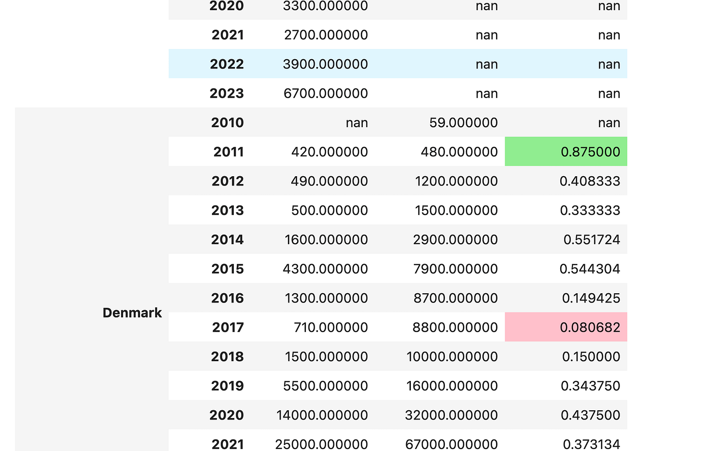
Once again, compare, for each year, the "stock" value with the "sales" value for cars with BEV powertrains. Add a column, "sales_pct_stock", showing the percentage of the stock that was sold. Wherever that percentage is >= 75%, color it light green. Wherever it's <= 10%, color it light red.]
Once again, we’ll start with our pivot table:
(
    df
    .loc[lambda df_: df_['parameter'].isin(['EV sales', 'EV stock'])]
    .loc[lambda df_: df_['powertrain'] == 'BEV']
    .pivot_table(index=['region', 'year'],
                columns='parameter',
                values='value')
)
We’ll then use “assign” to create a new column, “sales_pct_stock”, containing the sales divided by the stock:
(
    df
    .loc[lambda df_: df_['parameter'].isin(['EV sales', 'EV stock'])]
    .loc[lambda df_: df_['powertrain'] == 'BEV']
    .pivot_table(index=['region', 'year'],
                columns='parameter',
                values='value')
    .assign(sales_pct_stock=lambda df_:
            df_['EV sales'] / df_['EV stock'])
)
We now have the data we want. But I asked you to style it, highlighting some cells in green and others in red. To do that, we’ll need to use the “style” object. Every data frame has such an object, on which we can apply a number of different methods. You can change the foreground, background, highlighting, or even put a bar graph behind the text.
In this case, I decided to use the “highlight_between” method, which lets us say that if the value in a cell is between two states values (“left” and “right”), we want to color it in a particular way. And because “highlight_between” returns a “styler” object, we can then run “highlight_between” again on its output.
Here’s what I did:
(
    df
    .loc[lambda df_: df_['parameter'].isin(['EV sales', 'EV stock'])]
    .loc[lambda df_: df_['powertrain'] == 'BEV']
    .pivot_table(index=['region', 'year'],
                columns='parameter',
                values='value')
    .assign(sales_pct_stock=lambda df_:
            df_['EV sales'] / df_['EV stock'])
    .style
    .highlight_between(subset=['sales_pct_stock'],
                       left=0.75,
                       right=float('inf'),
                       color='lightgreen')
    .highlight_between(subset=['sales_pct_stock'],
                       left=float('-inf'),
                       right=0.10,
                       color='pink')
)
Note that while I said “light red” in the instructions, it turns out that the color system doesn’t recognize such a name. I renamed it “pink”, and I got the right kind of result. For example, here is a screenshot from the middle of my output:
That’s it for this week! I’m still traveling for another week, seeing some family and also meeting with some in-person corporate training clients. But you can be sure that I’ll have a new edition of Bamboo Weekly on Wednesday.
Meanwhile, here’s a link to my Jupyter notebook: https://drive.google.com/file/d/1XDXbI1ZCoALZPYfVLff80_DbXWMuNac2/view?usp=sharing
Until next week,
Reuven