


This week, we looked at the latest “World Economic Outlook” report from the International Monetary Fund (IMF, https://imf.org) on the world economy, giving both historical data and future projections on a variety of economic topics. They issued a complete report, as well as an executive summary, which were extensively covered by a variety of publications. You can read all about it, including downloading those written reports, here: https://www.imf.org/en/Publications/WEO/Issues/2024/04/16/world-economic-outlook-april-2024.
As data people, the reports aren’t as engaging as the underlying data. Fortunately, the IMF supplies all of the data that they used, allowing us to look at individual countries and also compare across them.
I decided to examine how members of the G20 (19 countries, plus the EU and the African Union — demonstrating that economists are also subject to off-by-one errors) have looked over the last few years. In particular, I wanted to better understand how well these countries have done in the last few years of post-pandemic economic weirdness.
Data and seven questions
The data we used was mainly from the IMF’s download page for their database:
https://www.imf.org/en/Publications/WEO/weo-database/2024/April/download-entire-database
Here are the seven tasks and questions that I gave you. A link to the Jupyter notebook I used to solve the problems is at the end of this post.
It takes 6-8 hours to research and write each edition of Bamboo Weekly. Thanks to those of you who support my work with a paid subscription! Even if you can’t, it would mean a lot if you would share BW with your Python- and Pandas-using colleagues. Thanks!
Download the full database from the IMF. If you're like me, you'll find that you have to jump through a number of hoops in order to get it loaded into Pandas. (I've never seen anything like this before, to be honest, and I'm surprised that the IMF distributed such a weird file.) Create the data frame such that it has a multi-index made up of the "Country" and "Subject Descriptor" columns, and the dtype of every column with a year heading is a float type.
Let’s start with the easiest thing, namely loading up Pandas:
import pandas as pdLoading up the file shouldn’t be a problem. We just go to the IMF’s site, click on the link, get a file, and we’re off to the races, right?
No. In this case, OMG, definitely not. The “download entire database” page offers the chance to download the file in tab-delimited format. I somehow missed that, downloaded the file, and saw that it had an “xls” extension, meaning Excel. I thus decided to use “read_excel” to read it into Pandas and got an error.
At first, I thought that it was because the version of Excel file they were using wasn’t right for my version of Pandas. I tried a few different Excel drivers, and none of them worked. Different libraries, such as “openpyxl” and “xlrd”, can handle different formats and problems with those formats. In this case, I struck out completely.
Hmm, I thought — maybe it’s really a CSV file, or it’s somehow tab-delimited? I looked at it, and even used the Unix “file” command, and both made it very clear that we’re talking about a binary file that is very much not in CSV format.
I thought that maybe things would be better or easier if I were to copy the link from the site, downloading the file using “wget” or a similar program, rather than my browser. (Because, as you know, browsers are just awful at downloading files from the Web, right?) That file had an “ashx” extension, indicating that it was likely produced on-the-fly from an ASP.NET application. However, it contained precisely the same data.
So now what? I decided that it might be worth loading this weird file into Excel. I got a really weird warning:

That scared me off a bit, so I didn’t open the file. Instead, I renamed it to have an “.xlsx” extension, which is for more modern versions of Excel. However, Excel refused to open that file at all. It didn’t even give me a warning.
So I went back to the downloaded file, opening it with Excel, and clicking “Yes” to the warning dialog box. And whadaya know, it opened just fine. (I tried to upload the document to Google Sheets, it refused to open the file.)
I quickly used “save as” to save the file in Excel format to another filename, and was relieved to find that things then worked:
df = (pd
      .read_excel('new-WEOApr2024all.xls')
)
Well, they almost worked. Loading the data worked just fine; I got a data frame from this command. But the IMF decided to use the two-character string “--” to represent missing values. This meant that every column with numeric data, which should have had a dtype of “np.float64” actually had a dtype of “object”, which means that the values were treated as strings, because there was no way to convert them all to integers or floats.
I passed the “na_values” keyword argument to “read_excel”, telling it that in addition to such strings as “NA” and “NaN”, I wanted “--” to be treated as a NaN value:
df = (pd
      .read_excel('/Users/reuven/Downloads/new-WEOApr2024all.xls',
                   na_values=['--'])
     )
That worked! Suddenly, all of the columns with years for headings (i.e., the numeric data) had dtypes of “np.float64”, as should be the case.
Finally, I asked you to set the “Country” and “Subject Descriptor” columns as the index. This means creating a multi-index of more than one column. We can always set it later on, but it’s very convenient to do so when we’re reading the file in, with the “set_index” keyword argument:
df = (pd
      .read_excel('/Users/reuven/Downloads/new-WEOApr2024all.xls',
                   na_values=['--'])
      .set_index(['Country', 'Subject Descriptor'])
     )
We end up with a data frame containing 8,626 rows and 58 columns, and with dtypes that are what we expect and want:
WEO Country Code                  object
ISO                               object
WEO Subject Code                  object
Subject Notes                     object
Units                             object
Scale                             object
Country/Series-specific Notes     object
1980                             float64
1981                             float64
1982                             float64
1983                             float64
1984                             float64
1985                             float64
1986                             float64
1987                             float64
1988                             float64
1989                             float64
1990                             float64
1991                             float64
1992                             float64
1993                             float64
1994                             float64
1995                             float64
1996                             float64
1997                             float64
1998                             float64
1999                             float64
2000                             float64
2001                             float64
2002                             float64
2003                             float64
2004                             float64
2005                             float64
2006                             float64
2007                             float64
2008                             float64
2009                             float64
2010                             float64
2011                             float64
2012                             float64
2013                             float64
2014                             float64
2015                             float64
2016                             float64
2017                             float64
2018                             float64
2019                             float64
2020                             float64
2021                             float64
2022                             float64
2023                             float64
2024                             float64
2025                             float64
2026                             float64
2027                             float64
2028                             float64
2029                             float64
Estimates Start After            float64
dtype: object
Whew! It worked — but it really annoyed me that I spent so much time trying to do something that should be so trivial. Moreover, this required manual intervention, meaning that it’s inappropriate for an automated series of tasks.
Which five countries had the lowest inflation (i.e., "Inflation, average consumer prices" where the units are "Percent change") in 2023? (Is that necessarily good?) Which countries had the highest inflation in 2023?
Inflation is clearly higher than it was before the pandemic started. In many countries, it has gone down quite a bit in the last few years, though. I was thus curious to know where inflation stood across the world — which countries have the lowest inflation, and which have the highest?
The first thing we have to do is select those rows for which the “Subject Descriptor” is “Inflation, average consumer prices.” Normally, that wouldn’t be too hard — except that “Subject Descriptor” is now part of our multi-index, which means that we cannot simply compare its value with what we want.
We also cannot use “.loc” to retrieve the rows that we want, because “Subject Descriptor” is the inner part of our multi-index.
The solution is to use “xs”, which lets us retrieve based on any part (or parts) of a multi-index. We indicate the value that we want to match, as well as the level that we want to match on, specifying it either by number (starting with 0) or by name (if the multi-index components are named):
(
    df
    .xs('Inflation, average consumer prices',
        level='Subject Descriptor')
)
It turns out, though, that there are two rows in our data file for this measure, each with a different set of units. (Maybe I should have added “Units” as a third dimension in our multi-index!) We thus need to keep only those rows that have “Percent change” for “Units”, which I can do using a combination of “.loc” and “lambda”:
(
    df
    .xs('Inflation, average consumer prices',
        level='Subject Descriptor')
    .loc[lambda df_: df_['Units'] == 'Percent change']
)
We now have only the rows that are of interest to us. But I was interested in finding out about the year 2023. I can use square brackets to retrieve just that year:
(
    df
    .xs('Inflation, average consumer prices',
        level='Subject Descriptor')
    .loc[lambda df_: df_['Units'] == 'Percent change']
    [2023]
)
This returns a series. I could then use “sort_values” to get the values, then look at the top and bottom of that sorted series. However, we’ll have a bunch of NaN values in there. So we could first run “dropna” and then “sort_values” — but it’s easier in many ways just to run “nsmallest”:
(
    df
    .xs('Inflation, average consumer prices',
        level='Subject Descriptor')
    .loc[lambda df_: df_['Units'] == 'Percent change']
    [2023]
    .nsmallest()
)
We get the following results:
Country
Turkmenistan   -1.738
Yemen          -1.225
Seychelles     -1.035
Bahrain         0.075
China           0.228
Name: 2023, dtype: float64
If you’ve been living in an inflationary economy for a few years, this might sound great. Negative inflation (i.e., “deflation”) especially sounds terrific, right? Prices would fall each month, rather than rise.
But as good as deflation sounds, it’s actually pretty awful. Why would you buy something now, if you know that it’ll be cheaper next month, and much cheaper in a year? If everyone puts of buying things then the economy has a real problem getting jump-started.
Central banks want to limit inflation, but they typically don’t want it to go away completely. They keep talking about getting inflation levels to about 2 percent as a good balance, such that prices rise a bit, but not too much.
How about the most inflationary economies? If you’ve been complaining about inflation in your country, then you might well need to sit down before running this query, which uses “nlargest”:
(
    df
    .xs('Inflation, average consumer prices',
        level='Subject Descriptor')
    .loc[lambda df_: df_['Units'] == 'Percent change']
    [2023]
    .nlargest()
)
The results:
Country
Zimbabwe     667.361
Venezuela    337.458
Sudan        171.471
Argentina    133.489
T¸rkiye       53.859
Name: 2023, dtype: float64
That’s pretty darned high. Turkey — often written as Türkiye, whose “ü” didn’t survive the transformation of file formats — had a very high rate of inflation last year, which many were sure would affect their presidential election, but didn’t. Argentina’s rate is even higher (133 percent!), which almost certainly did help Javier Milei to win the presidency there.
Here’s a fantastic story from NPR about how Brazil conquered hyperinflation a number of years ago using a fake currency: https://www.npr.org/sections/money/2010/10/01/130267274/the-friday-podcast-how-four-drinking-buddies-saved-brazil
Create a list, series, or NumPy array containing the names of G20 countries. One good source is https://en.wikipedia.org/wiki/G20, which lists them all. Remember that the G20 has 19 country members. plus two unions of countries -- the European Union and the African Union. Remove any extraneous characters.
Because I want to focus on G20 countries, we’ll need to get a list of those countries. One of my favorite techniques for retrieving data from a Web page is “read_html”, which returns a list of data frames, each containing data from an HTML table. So a page with five tables will return a list of five data frames, while a page with 10 tables will return a list of 10 data frames.
I found that I could easily get the G20 members’ names from the third table (i.e., index) on Wikipedia, so I used this code:
g20_url = 'https://en.wikipedia.org/wiki/G20'

g20_names = (pd
          .read_html(g20_url)[2]
          ['Member']
         )
This returns a series of strings, each a member of the G20. However, we got duplicates of several country names, because the “Member” column spanned two entries in the “Leader” column for China, the European Union, and the African Union. The latter two won’t be a problem for us, because neither union appears in the IMF data — but the duplicate China will be. So, I called “drop_duplicates” to return a series without any duplicated names:
g20_url = 'https://en.wikipedia.org/wiki/G20'

g20_names = (pd
          .read_html(g20_url)[2]
          ['Member']
          .drop_duplicates()
         )
Next, I wanted to remove the footnotes from the names. To be honest, this might be unnecessary, because neither the EU nor the AU will be in the IMF’s data. That said, you can never have too many regular expressions, right? Here, I search for:
- A literal [ character, specified as \[
- One or more decimal digits, specified as \d+
- A literal ] character, specified as \]
These are all inside of a raw string, to ensure the backslashes are themselves escaped. I then feed this to “str.replace”, making sure to indicate that regex=True, so that the search string will be interpreted as a regular expression:
g20_url = 'https://en.wikipedia.org/wiki/G20'

g20_names = (pd
          .read_html(g20_url)[2]
          ['Member']
          .drop_duplicates()
          .str.replace(r'\[\d+\]', '', regex=True)
         )
We now have a Pandas series containing the G20 members:
0              Argentina
1              Australia
2                 Brazil
3                 Canada
4                  China
6                 France
7                Germany
8                  India
9              Indonesia
10                 Italy
11                 Japan
12                Mexico
13                Russia
14          Saudi Arabia
15          South Africa
16           South Korea
17                Turkey
18        United Kingdom
19         United States
20    European Union[62]
22         African Union
Name: Member, dtype: object
But wait: There’s a small-but-significant issue with our data. Notice that at index 16, we have the country named “South Korea.” That’s fine, except that in the IMF’s data, it’s named just “Korea”. (I’m guessing that this is because North Korea doesn’t participate in the IMF, but I don’t know for sure.)
To make sure that the data will match up, we can also replace any mention of “South Korea” with just “Korea”:
g20_names = (pd
          .read_html(g20_url)[2]
          ['Member']
          .drop_duplicates()
          .str.replace(r'\[\d+\]', '', regex=True)
          .str.replace('South Korea', 'Korea')
         )
We’re now ready to use our G20 names to analyze a subset of the IMF data.
Among members of the G20, who had the lowest inflation rate in 2023? Who had the highest?
We already found inflation rates among all countries. How can we find the rates among G20 countries?
The first thing we’ll do is retrieve only those rows from df whose outer index is in our “g20_names” series:
(
    df
    .loc[g20_names]
)
This returns a subset of df, only containing G20 data. We can then use “xs” and “.loc” as we did before, to get the percent change in inflation:
(
    df
    .loc[g20_names]
    .xs('Inflation, average consumer prices',
        level='Subject Descriptor')
    .loc[lambda df_: df_['Units'] == 'Percent change']
)
You might be wondering, by the way, why I didn’t use “.loc” to match both parts of the multi-index. So far as I can tell, there isn’t any way for that to work. If I wanted a specific range of values from the multi-index’s outer layer, then I could use a slice. But I wanted specific values from the multi-index, and that doesn’t seem to work.
There is an “IndexSlice” object that you can use, but it didn’t seem to make the queries any shorter or more intuitive. So I stuck with what I had here.
Next, I only wanted the year 2023, so I used square brackets:
(
    df
    .loc[g20_names]
    .xs('Inflation, average consumer prices',
        level='Subject Descriptor')
    .loc[lambda df_: df_['Units'] == 'Percent change']
    [2023]
)
I then called “sort_values” on our series:
(
    df
    .loc[g20_names]
    .xs('Inflation, average consumer prices',
        level='Subject Descriptor')
    .loc[lambda df_: df_['Units'] == 'Percent change']
    [2023]
    .sort_values()
)
Here’s the result of this query:
Country
China               0.228
Saudi Arabia        2.327
Japan               3.268
Korea               3.593
Indonesia           3.713
Canada              3.879
United States       4.128
Brazil              4.594
India               5.375
Mexico              5.525
Australia           5.595
France              5.662
Russia              5.859
South Africa        5.900
Italy               5.903
Germany             6.030
United Kingdom      7.306
Argentina         133.489
Name: 2023, dtype: float64
We thus see that in 2023, China had the lowest rate of inflation, while Argentina had (by far!) the highest rate.
Create a bar plot showing all G20 members' inflation rates from 2019 through 2023, with one cluster of bars per country and one bar per year. If the plot gets unreadable due to outlier values, remove that outlier before plotting. Sort by 2023 inflation figures. Does any year stick out in particular? Why?
I then asked you to plot the G20 inflation over the last few years. The query starts much the same as the previous one, but I asked you to plot a range of years, not just 2023. For that, I can use a range object inside of square brackets, to retrieve only a subset of columns:
(
    df
    .loc[g20_names]
    .xs('Inflation, average consumer prices',
        level='Subject Descriptor')
    .loc[lambda df_: df_['Units'] == 'Percent change']
    [range(2019, 2024)]
)
I can then use “sort_values” to sort by the values in 2023, and then use “plot.bar” to create a bar plot:
(
    df
    .loc[g20_names]
    .xs('Inflation, average consumer prices',
        level='Subject Descriptor')
    .loc[lambda df_: df_['Units'] == 'Percent change']
    [range(2019, 2024)]
    .drop('Argentina')
    .sort_values(2023)
    .plot.bar()
)
And here’s the plot we get:
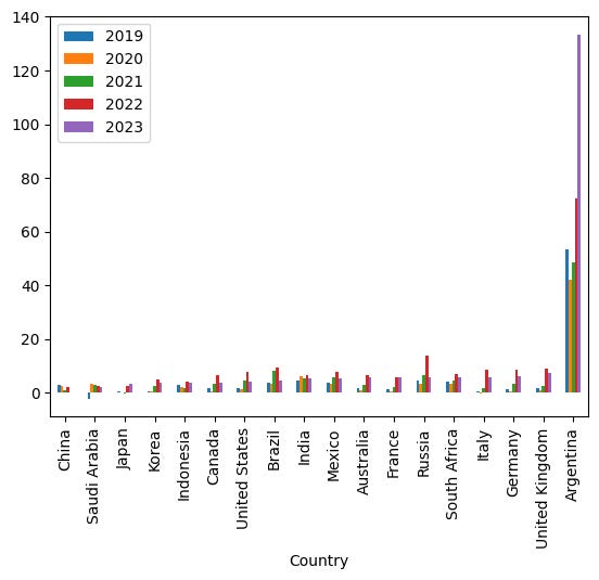
So… it isn’t wrong, per se. But Argentina has so much more inflation than other members of the G20 that it makes the graph pretty much unusable. I thus decided to use “drop” to remove Argentina, and I tried again:
(
    df
    .loc[g20_names]
    .xs('Inflation, average consumer prices',
        level='Subject Descriptor')
    .loc[lambda df_: df_['Units'] == 'Percent change']
    [range(2019, 2024)]
    .drop('Argentina')
    .sort_values(2023)
    .plot.bar()
)
Here’s what I got this time around:
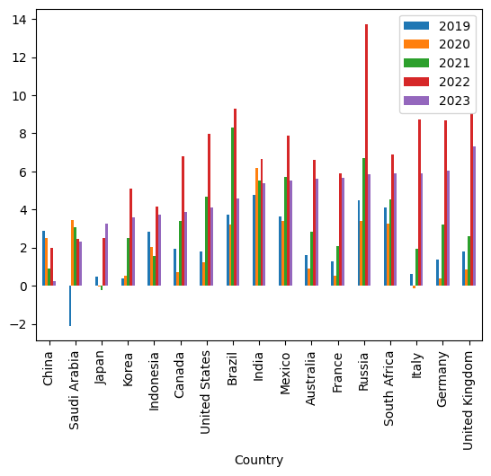
According to this data, the countries with the lowest inflation in the G7 are China, Saudi Arabia, Japan, Korea, Indonesia, and Canada, with the US coming up next. By contrast, we see that Italy, Germany, and the UK have the highest inflation in the G7, with the UK’s rate clocking in at about 1.5 percent higher than Germany — as we saw in the numeric data from the previous question.
As for a year that sticks out, that would be 2022, when the effects of restarting every economy in the world at the same time, along with giving various types of economic stimulus to businesses and individuals, started to be felt in earnest.
For each country in the G20, calculate the "misery index" (https://en.wikipedia.org/wiki/Misery_index_(economics)), the combination of inflation and unemployment. Create a bar plot, again showing the years 2019-2023 for each country, and sorted by the misery-index calculation for each country.
The “misery index” combines inflation and unemployment to find out how unhappy a country’s population is.
We’ll once again start by restricting our query to the G20:
(
    df
    .loc[g20_names]
)
After wrestling with this data for a little while, I decided that yes, I could still use “xs” to retrieve two different subjects, but that it was just too annoying and clunky. So I instead to use “reset_index”, along with the “level” keyword argument, to return it to being a regular column:
(
    df
    .loc[g20_names]
    .reset_index(level="Subject Descriptor")
)
With that in place, I was then able to use “.loc” to keep only those rows where the “Subject Decriptor” was either the unemployment rate or inflation, using “isin” on those strings:
(
    df
    .loc[g20_names]
    .reset_index(level="Subject Descriptor")
    .loc[lambda df_:
         df_['Subject Descriptor'].isin(
             ['Unemployment rate',
              'Inflation, average consumer prices'])]
)
The thing is, this isn’t enough: As we’ve seen before, we also need to choose the right rows based on the units measured. And here, we only wanted percentages. I decided to use “.loc” to keep only those rows in which “Units” started with the string “Percent”, using “str.startswith”:
(
    df
    .loc[g20_names]
    .reset_index(level="Subject Descriptor")
    .loc[lambda df_:
         df_['Subject Descriptor'].isin(
             ['Unemployment rate',
              'Inflation, average consumer prices'])]
    .loc[lambda df_: df_['Units'].str.startswith('Percent')]
)
Now I can restrict the columns to only the years 2019-2013, using range:
(
    df
    .loc[g20_names]
    .reset_index(level="Subject Descriptor")
    .loc[lambda df_:
         df_['Subject Descriptor'].isin(
             ['Unemployment rate',
              'Inflation, average consumer prices'])]
    .loc[lambda df_: df_['Units'].str.startswith('Percent')]
    [range(2019, 2024)]
)
But now what? We now have two rows per country, and we want to add them together, on a per-country basis. This seems like a great time to use “groupby”:
(
    df
    .loc[g20_names]
    .reset_index(level="Subject Descriptor")
    .loc[lambda df_:
         df_['Subject Descriptor'].isin(
             ['Unemployment rate',
              'Inflation, average consumer prices'])]
    .loc[lambda df_: df_['Units'].str.startswith('Percent')]
    [range(2019, 2024)]
    .groupby('Country').sum()
)
The result is a data frame in which the index contains G2 country names, and each of the four columns contains the misery index for each country in that year. We can now sort them by 2023 values, and plot:
(
    df
    .loc[g20_names]
    .reset_index(level="Subject Descriptor")
    .loc[lambda df_:
         df_['Subject Descriptor'].isin(
             ['Unemployment rate',
              'Inflation, average consumer prices'])]
    .loc[lambda df_: df_['Units'].str.startswith('Percent')]
    [range(2019, 2024)]
    .groupby('Country').sum()
    .sort_values(2023)
    .plot.bar()
)
Here’s the result:
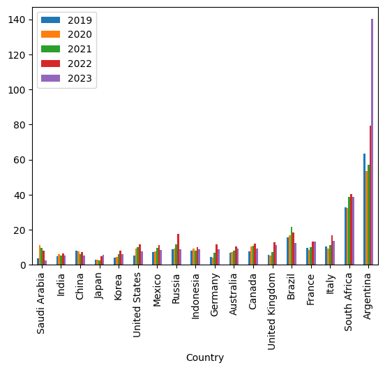
Let’s (again) remove Argentina to get a better sense of things:
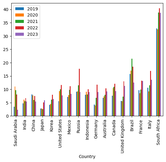
We see that South Africa had a very high misery index last year, followed (not too closely) by Italy, France, and Brazil, whereas Saudi Arabia, India, and China seemed to be doing pretty well on that front.
Finally, let's look at the predicted change in GDP for G20 countries this year. Grab the "Gross domestic product, constant prices" descriptor with "Percent change" for 2024. Which countries will grow the least? Which will grow the most?
Who is projected to do best this year? Let’s take a look, first grabbing G20 countries and then looking at GDP in constant prices with a percent change:
(
    df
    .loc[g20_names]
    .xs('Gross domestic product, constant prices',
         level='Subject Descriptor')
    .loc[lambda df_: df_['Units'] == 'Percent change']
)
Next, I asked for only 2024:
(
    df
    .loc[g20_names]
    .xs('Gross domestic product, constant prices',
         level='Subject Descriptor')
    .loc[lambda df_: df_['Units'] == 'Percent change']
    [2024]
)
Next, I sorted the values:
(
    df
    .loc[g20_names]
    .xs('Gross domestic product, constant prices',
         level='Subject Descriptor')
    .loc[lambda df_: df_['Units'] == 'Percent change']
    [2024]
    .sort_values()
)
The results:
Country
Argentina        -2.764
Germany           0.150
United Kingdom    0.460
Italy             0.709
France            0.744
Japan             0.855
South Africa      0.879
Canada            1.154
Australia         1.461
Brazil            2.154
Korea             2.322
Mexico            2.367
Saudi Arabia      2.554
United States     2.725
Russia            3.163
China             4.642
Indonesia         4.964
India             6.808
Name: 2024, dtype: float64
Yikes — it looks like Argentina is in for a pretty rough year, with a contraction of their economy. By contrast, we see that India is in for a sizzling year of growth, at 6.8 percent. The US is on track to grow very nicely for a developed economy, at 2.7 percent. But how, given its invasion of Ukraine and trade restrictions, is Russia poised to grow at more than 3.1 percent? And how, with its economic issues, will China grow at 4.6 percent? Given that dozens (maybe hundreds) of professional economists worked on this projection, I’ll assume that they know what they’re talking about — but at the same time, economics is far from perfect at making predictions.
That’s it for this week!
Here’s a link to my Jupyter notebook: https://drive.google.com/file/d/1pATGipqGlXvkGvwpTwfVJTeMyy3Nl4pY/view?usp=sharing
I’ll be back with more puzzles about Python and Pandas, taken from current events, next week.
Reuven