Bamboo Weekly #46: Pedestrians (solutions)

This week, we looked at the US Department of Transportation’s data on car accidents, and specifically pulled information out about those involving pedestrians. The goal was to get a better sense of how many such accidents occur, when and where they occur, and whether they have indeed been rising over the last few years.

This topic was inspired by something that I’ve seen reported several times in the last few weeks, most notably in the New York Times (https://www.nytimes.com/interactive/2023/12/11/upshot/nighttime-deaths.html?unlocked_article_code=1.JE0.6nDD.DwDlgNGWvbej&smid=url-share), but also on Slate's Political Gabfest (https://slate.com/podcasts/political-gabfest/2023/07/extreme-weather-heat-and-floods-are-killing-us-political-gabfest), and in a Vox article (https://www.vox.com/23784549/pedestrian-deaths-traffic-safety-fatalities-governors-association).

And then, just last (Wednesday) night, I was reading “The Phoenix Economy” by Felix Salmon, in which he talks about this topic as part of a general discussion of risk, and how people re-thought it during the pandemic.

Since hearing about “stroads” (https://en.wikipedia.org/wiki/Stroad) and their influence on urban life in the United States, I’ve taken greater notice of how different cities are constructed, and how that affects our ability to get around on foot vs. by car.

Data and six questions

This week’s data comes from the "Fatality Analysis Reporting System" (FARS), part of the National Highway Traffic Safety Administration, which is itself part of the US Department of Transportation. The FARS home page is at:

https://www.nhtsa.gov/research-data/fatality-analysis-reporting-system-fars

The data is all available from the following site:

https://www.nhtsa.gov/content/nhtsa-ftp/251

That site (which then redirects to another URL) contains a folder for each year of FARS data, starting in 1975 and going through 2021. Inside of each year’s folder is a sub-folder called “National.” And inside of the “National” folder, you’ll see a file named FARSYYYYNationalCSV.zip, where YYYY is the year for which the data was collected.

The (very long) data dictionary that describes most (but not all!) of the columns in the data we'll be looking at is here:

https://crashstats.nhtsa.dot.gov/Api/Public/ViewPublication/813426

This week, I gave you six questions and tasks for working with this data set. Most weeks, it’s fairly straightforward to load the data into a data frame — but this week, loading the data turned out to be the most difficult and complex part. But hey, that’s the way it often is with data analysis; importing and cleaning the data can often be harder than the analysis itself.

Here are my solutions to this week’s questions. As always, a link to the Jupyter notebook I used to solve these problems is at the bottom of this post. And given the complexity of what we’re doing this week, I expect more than ever to get suggestions and feedback on my solutions.

Create two data frames from the FARS data in 2021, one for accidents and one for people. Use the `requests` package (https://docs.python-requests.org/en/latest/index.html) plus the `zip` and `BytesIO` modules in Python's standard library to retrieve and process these files, turning them into a data frame.

Let’s start by loading up Pandas, as well as several other modules that we’ll need:

• requests, from PyPI
• io.BytesIO, from the Python standard library
• zipfile, from the Python standard library

from zipfile import ZipFile
from io import BytesIO
import requests 

How can we use these together to download one file (say, from 2010) and turn it into a data frame?

Well, we can download the data via requests:

url = f'https://static.nhtsa.gov/nhtsa/downloads/FARS/2010/National/FARS2010NationalCSV.zip'

b = requests.get(url).content

The above returns a bytestring (aka “bytes”), a core Python data structure that contains individual 8-bit bytes. It’s easy to confuse this with ASCII characters, because ASCII was a one-byte encoding, where every character used one and only one byte. The good news is that this was easy to work with; the bad news was that it excluded most non-English languages, which rumor has it they speak in some countries. You shouldn’t think of a bytestring as characters, but rather as individual integers that can be turned into characters (i.e., a string) if and when we want.

Whenever we ask for “content” from requests, we always get a bytestring back. If the bytestring contains text, then we can turn it into a regular string with the “decode” method, but (as we’ll discuss in a bit) this can be tricky. But right now, our bytestring contains a zipfile, which is most definitely not text.

How can we read from the zipfile? We can use the “ZipFile” class from the “zipfile” module, handling it as a file and then extracting whatever is interesting to us. But we can’t quite do that yet, because ZipFile expects to get a file, and our bytestring is most definitely not a file.

Actually, ZipFile doesn’t really expect to get a file. Rather, it wants to get what we in the Python world call a “file-like object,” meaning something that implements the same API as a file. If you want to construct such an object from a string, simulating a text file, you can use io.StringIO. And if you want to do the same thing with bytes, then you can use io.BytesIO:

zipfile_contents = BytesIO(requests.get(url).content)

Here, we create a BytesIO object based on what we got back from requests. We can then use ZipFile on it. But then what?

One option is to extract the files that we got in the zipfile, and then read through those files on disk. But we can be much more elegant than that, taking advantage of ZipFile’s implementation of the context manager protocol — meaning, simply put, that we can put it in a “with” block. Then we can perform all sorts of actions on the zipfile and its contents without actually touching the filesystem:

    with ZipFile(zipfile_contents) as myzip:

Fine, but what should be inside of the “with” block? Basically, we want to find two files, “accident.csv” and “person.csv”. Sadly, these files might come in all sorts of weird combinations of capitalization, which makes it harder to find the file. However, we can be a bit clever, and do the following:

• Get the list of files in the zipfile with myzip.namelist()
• Iterate through each of those files, looking for accident.csv or person.csv, or anything looking roughly like them
• If we find a match, then we set that to be the CSV filename we want to work with
• If we don’t find any match, then we give an error message, and try again.

That sounds nice, but how can we look for filenames “or anything looking roughly like them”?

The answer is simple: Regular expressions, which allow us to search for patterns of text. If you find yourself using “if” with many different possible variations, but you can describe the text you’re trying to find with a single English sentence, then a regular expression might well help you.

Here’s what I did in my code to find accident.csv and person.csv, ignoring whatever crazy capitalization they decided to use in that particular reporting year:

        for basename in ['accident', 'person']:

            for one_filename in myzip.namelist():
                if re.search(f'{basename}\.csv', one_filename, re.I):
                    print(f'Matched {one_filename}')
                    csv_filename = one_filename
                    break
    
            else:
                print(f'No match; names are: {myzip.namelist()}')

In other words:

• Iterate over each of “accident” and “person”, calling it “basename”
• Go through each filename in the zipfile’s contents
• Check to see if “basename” followed by “.csv”, ignoring capitalization, matches the word. I use “re.search” here, because it gives us the most flexibility.
• I pass the “re.I” flag, indicating that I want the search to be case-insensitive
• If I find a match, then I assign it to “csv_filename” and then break out of the for loop

Notice the “else” after the “for”? That’s a great Python feature that is also a bit confusing. Basically, that “else” will fire if we reach the end of the “for” loop without encountering a “break”. In other words: We went through all of the options, and none of them seemed to fit.

I have a YouTube video on this subject, if you want to learn more:

With the filenames in hand, we can then create data frames. In theory, we would like to do something as simple as this:

df = pd.read_csv(csv_filename)

But there are at least three problems with this:

• First, I discovered (the hard way!) that these CSV files don’t use Unicode. That is, trying to read from these CSV files directly into a text file, string, or data frame won’t work. That’s because the files were written using a one-byte encoding known as Latin-1 that covers all ASCII characters (in bytes 0-127) and then many Western European languages (in bytes 128-255). Latin-1 was very popular for many years, and covered the majority of Western countries. But because it uses the top half of each byte, it’s incompatible with Unicode, and cannot be read that way. However, if we specify the encoding to “open” or “read_csv”, then we’re fine.
• Some of the data files are also long enough that Pandas needs to break them up into chunks before analyzing them and deciding what dtype to assign to each column. This can result in some mismatches and/or warnings from Pandas indicating that the dtypes might be wrong. To avoid this, you can pass “low_memory=False” as a keyword argument. This will use more RAM, but it’ll run faster and give a more accurate assessment.
• Finally, remember that we’re inside of a “with” block on the ZipFile, which I’ve called “myzip”. If we want to read the file without actually extracting it, we can use “myzip.open”.

Given all that, we can use the following combination of code to open the CSV file, read it into a data frame, and assign that data frame to a variable:

            with myzip.open(csv_filename) as csv_file:
                df = pd.read_csv(csv_file,
                                 encoding='Latin-1',
                                 low_memory=False))

Repeating that for each of our two CSV files will do the trick.

When you have that working, now create two data frames, `accident_df` and `person_df`, based on all of the data from 2010 through 2021.

The above was fine for turning one or two files into data frames. But we need to repeat this (on each of the two CSV files) for each of the years. How can we do that?

Here’s my basic plan:

• I’ll create a dictionary, “all_dfs”, with two keys (“accident” and “person”), each of whose values is an empty list.
• I’ll then iterate through each year we want to examine with “range”, building a URL that we download with requests and turn into a BytesIO.
• We can then use the above code to find the matching filename (using regular expressions), reading the CSV file into a data frame, and appending that data frame to the appropriate list in “all_dfs”
• Finally, we can call “pd.concat” on each of the lists, resulting in a single data frame that’s the result of combining/merging all of the downloaded data.

Here’s the code that I wrote and used, including a bunch of “print” statements to keep track of what’s happening:

from zipfile import ZipFile
from io import BytesIO
import requests 
import re

all_dfs = {'accident': [],
          'person':[]}

for year in range(2012, 2022):
    url = f'https://static.nhtsa.gov/nhtsa/downloads/FARS/{year}/National/FARS{year}NationalCSV.zip'
    print(url)

    zipfile_contents = BytesIO(requests.get(url).content)

    with ZipFile(zipfile_contents) as myzip:
    
        for basename in ['accident', 'person']:

            for one_filename in myzip.namelist():
                if re.search(f'{basename}.csv', one_filename, re.I):
                    print(f'Matched {one_filename}')
                    csv_filename = one_filename
                    break
    
            else:
                print(f'No match; names are: {myzip.namelist()}')
            
            with myzip.open(csv_filename) as csv_file:
                all_dfs[basename].append(pd.read_csv(csv_file,
                                                    encoding='Latin-1',
                                                    low_memory=False))
    
accident_df = pd.concat(all_dfs['accident'])
person_df = pd.concat(all_dfs['person'])

At the end of this process, we have two data frames, one from each of the CSV collections:

• accident_df, with 335,959 rows and 92 (!) columns, and
• person_df, with 828,742 rows and 172 (!!) columns

And yes, if we were interested in saving memory, we would definitely be choosier about the columns that we load, rather than creating such ridiculously wide data frames. I decided that they were small enough for most modern computers, and didn’t want to make the above code even more complex by suggesting that you pass a value to the “usecols” keyword argument.

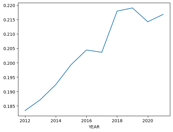
What percentage of the accidents, per year, involve a pedestrian? Is that percentage increasing from year to year?

Next, I asked you to find the percentage of accidents that involve a pedestrian. In accident_df, the PEDS column indicates the number of pedestrians that were involved in an accident. If we can find out how often PEDS was not 0 in a given year, then we can use that to calculate and compare.

Let’s step back for a moment and ask a broader question: What if we want to find out the percentage of accidents that involved a pedestrian across all years? For that, we could use my favorite method, “value_counts”, which tells us how often a value appears in a column. By passing “normalize=True” as a keyword argument, we get the percentage, rather than the number. We can thus say:

(
    accident_df
    ['PEDS']
    .value_counts(normalize=True)
)

That’s fine, but it shows us the percentage for all number of pedestrians. I want the total percentage for accidents with a non-zero number of pedestrians. Fortunately, teh result of value_counts is a series. We can drop the row with 0 as an index (using “drop”), sum up the remaining values, and then round to the nearest hundredths digit:

(
    accident_df
    ['PEDS']
    .value_counts(normalize=True)
    .drop(0)
    .sum()
    .round(2)
)

I get a result of 0.2, which tells us that across the entire data set, 20 percent of accidents involve pedestrians.

But of course, I don’t want to know across the entire data set; I want to know the percentage per year. Given that value_counts is an aggregation method, we can apply it to the result of a “groupby” operation:

(
    accident_df
    .groupby('YEAR')['PEDS']
    .value_counts(normalize=True)
)

The result is a series with a two-level multi-index. The outer level of the index contains the years, and the inner level contains the number of pedestrians involved in accidents.

We again want to remove all of the entries with 0 pedestrians. Here, I think that we’ll be well served by using “unstack”, which takes the inner part of the multi-index and turns it into column names. The result is a data frame in which the years are the rows (index) and the number of pedestrians are the columns.

(
    accident_df
    .groupby('YEAR')['PEDS']
    .value_counts(normalize=True)
    .unstack()
)

Now we can remove column 0 using “drop”, indicating that we want to drop a column:

(
    accident_df
    .groupby('YEAR')['PEDS']
    .value_counts(normalize=True)
    .unstack()
    .drop(0, axis='columns')
    .sum(axis='columns')
)

Finally, we sum across the columns, giving us a total percentage of accidents involving pedestrians for each year:

(
    accident_df
    .groupby('YEAR')['PEDS']
    .value_counts(normalize=True)
    .unstack()
    .drop(0, axis='columns')
    .sum(axis='columns')
)

Here’s what I get:

YEAR
2012    0.183352
2013    0.187173
2014    0.192374
2015    0.199305
2016    0.204415
2017    0.203617
2018    0.217931
2019    0.219040
2020    0.214220
2021    0.216792
dtype: float64

It looks like the numbers are basically increasing, but are they? We can add a call to “pct_change” to find out how much each year’s value is different from the previous year:

(
    accident_df
    .groupby('YEAR')['PEDS']
    .value_counts(normalize=True)
    .unstack()
    .drop(0, axis='columns')
    .sum(axis='columns')
    .pct_change()
)

The result:

YEAR
2012         NaN
2013    0.020842
2014    0.027788
2015    0.036030
2016    0.025635
2017   -0.003903
2018    0.070299
2019    0.005090
2020   -0.022006
2021    0.012004
dtype: float64

So yes, it would seem that over the last 10 years, in all but two years the percentage of accidents involving a pedestrian has increased.

I should add that there’s at least one other way to solve this problem: After unstacking, and getting a data frame with years as rows and number of pedestrians as columns, we could keep only the 0 column. Then we could use “lambda” to apply a simple function to that column, subtracting 1 from its value. That gives the same result, and assumes that the percentages will add up to 1.00 (or close to it):

(
    accident_df
    .groupby('YEAR')['PEDS']
    .value_counts(normalize=True)
    .unstack()
    [0]
    .apply(lambda s: 1 - s)
    .pct_change()
)

Plotting this sort of thing is always more striking; if I want to visualize the percentage of accidents involving a pedestrian (not the percentage change), I can use the following code:

(
    accident_df
    .groupby('YEAR')['PEDS']
    .value_counts(normalize=True)
    .unstack()
    [0]
    .apply(lambda s: 1 - s)
    .plot.line()
)

This results in the following plot:

Under what light conditions did accidents involving pedestrians occur?

One of the conclusions in the New York Times article was that pedestrian accidents weren’t increasing during the day, but they were increasing — dramatically — at night. Let’s take an initial look at this data, looking only at accidents involving pedestrians, and finding how often each light condition applied.

First, I only want the rows from “accident_df” in which the value of PEDS is not 0. I can use “loc” to filter those out:

(
    accident_df
    .loc[
      accident_df['PEDS'] > 0, 
      'LGT_CONDNAME']
)

Remember that loc can take one argument (a row selector) or two arguments (a row selector, followed by a column selector). Here, I chose rows where the value of PEDS is greater than 0, and I chose the “LGD_CONDNAME” column. And yes, I did tell you in the original instructions to look at “LGT_COND”, but that’s because I forgot that it contained integers, and that the LGT_CONDNAME column contained text strings that we can interpret and understand.

With that series in place, I can again call value_counts, passing normalize=True:

(
    accident_df
    .loc[
      accident_df['PEDS'] > 0, 
      'LGT_CONDNAME']
    .value_counts(normalize=True)
)

Here’s what I get:

LGT_CONDNAME
Dark - Lighted             0.370648
Dark - Not Lighted         0.328238
Daylight                   0.245239
Dusk                       0.020595
Dawn                       0.016933
Dark - Unknown Lighting    0.012903
Not Reported               0.002015
Reported as Unknown        0.001724
Unknown                    0.000911
Other                      0.000794
Name: proportion, dtype: float64

Not surprisingly, we see that when it’s dark (lighted, not lighted, or unknown) is when about 70 percent of accidents involving pedestrians occur. I was surprised to find that there are more accidents when it’s dark and there is light around; whether that’s because people are complacent, or because it’s along those “stroads” that inherently attract both people and cars, isn’t obvious to me.

If an accident involves a pedestrian, what percentage of the time does it result in a death or serious injury?

How often do accidents result in death or serious injury? We can turn to person_df, which has information about people involved in accidents, and check the INJ_SEV (or, as I should have said in my original instructions, INJ_SEVNAME, which gives us the text rather than numeric codes).

Let’s see how often each injury severity shows up:

(
    person_df['INJ_SEVNAME']
    .value_counts(normalize=True)
)

I get these results:

INJ_SEVNAME
Fatal Injury (K)                0.440038
No Apparent Injury (O)          0.251284
Possible Injury (C)             0.081615
Suspected Minor Injury (B)      0.076127
Suspected Serious Injury (A)    0.074234
Suspected Minor Injury(B)       0.031364
Suspected Serious Injury(A)     0.028334
Unknown/Not Reported            0.012845
Injured, Severity Unknown       0.002820
Unknown                         0.001312
Died Prior to Crash*            0.000026
Name: proportion, dtype: float64

We can see that there are several repeats among these values, thanks in no small part to inconsistent tagging. Let’s remove the space, parentheses, and single-letter codes from after the descriptions, using a regular expression in the “str.replace” method:

(
    person_df['INJ_SEVNAME']
    .str.replace('\s*\(\w\)\s*', '', regex=True)
    .value_counts(normalize=True)
)

The above regular expression means:

• Zero or more whitespace characters, \s*
• A single alphanumeric character in between parentheses, \(\w\)
• Zero or more whitespace characters, \s*

We replace any occurrence of such a pattern with the empty string, and tell str.replace that we’re using a regular expression with “regex=True”. The result:

INJ_SEVNAME
Fatal Injury                 0.440038
No Apparent Injury           0.251284
Suspected Minor Injury       0.107491
Suspected Serious Injury     0.102568
Possible Injury              0.081615
Unknown/Not Reported         0.012845
Injured, Severity Unknown    0.002820
Unknown                      0.001312
Died Prior to Crash*         0.000026
Name: proportion, dtype: float64

We can now grab only those rows whose indexes mention “fatal” or “serious” injuries:

(
    person_df['INJ_SEVNAME']
    .str.replace('\s*\(\w\)\s*', '', regex=True)
    .value_counts(normalize=True)
    .loc[['Fatal Injury', 'Suspected Serious Injury']]
)

We get the following result:

INJ_SEVNAME
Fatal Injury                0.440038
Suspected Serious Injury    0.102568
Name: proportion, dtype: float64

If we now want to know the proportion of fatal or serious injuries, we just sum up these numbers:

(
    person_df['INJ_SEVNAME']
    .str.replace('\s*\(\w\)\s*', '', regex=True)
    .value_counts(normalize=True)
    .loc[['Fatal Injury', 'Suspected Serious Injury']]
    .sum()
    .round(2)
)

The result: 0.54, meaning that 54 percent of accidents involving pedestrians result in death or serious injury.

Wow. That’s a very high number, don’t you think? More than half of all accidents involving people result in a fatality or serious injury?

Does that really make sense? It’s possible, I guess, but seems a bit steep.

Consider this: person_df data frame counts all of the people involved in car accidents. Which means that we didn’t exactly count how many car accidents resulted in death or serious injury. Rather, we counted how many people involved in car accidents were killed or seriously injured.

For example, consider case number 480549. How many people were injured in this one accident, and how seriously were they injured? We can find out:

(
    person_df
    .loc[person_df['ST_CASE'] == 480549, "INJ_SEVNAME"]
    .value_counts()
)

Here’s the answer:

INJ_SEVNAME
Suspected Minor Injury (B)      66
No Apparent Injury (O)          31
Unknown/Not Reported            20
Suspected Serious Injury (A)    14
Fatal Injury (K)                12
Possible Injury (C)              7
Name: count, dtype: int64

So our analysis is good, but I think it could be better.

What if we instead want to find the proportion of accidents in which someone was killed or seriously injured? We would have to find all of the accidents with fatal or serious injuries. Then we could grab ST_CASE (i.e., the case numbers), drop the duplicates, and count how many distinct case numbers had these sorts of injuries. Then we could divide that number by the total number of cases:

(
    person_df
    .loc[person_df['INJ_SEV'].isin([3, 4]),
         'ST_CASE']
    .drop_duplicates()
    .count()
    / person_df['ST_CASE'].count()
).round(2)

First, we find all of the rows in which INJ_SEV (the numeric codes for fatality or serious injury, 3 or 4) using “isin”. We only grab the ST_CASE column based on that.

Then we remove duplicates from that series, count how many unique values there are, and divide that by the total number of values in ST_CASE.

Finally, we round to the hundredths digit, and get a result of: 0.05, or 5 percent.

In other words, there are fatalities and serious injuries in just 5 percent of the auto accidents. Which is still a large number, but it’s a far cry from 54 percent.

Of course, I might have misinterpreted this as well; if you have additional analysis, please share it.

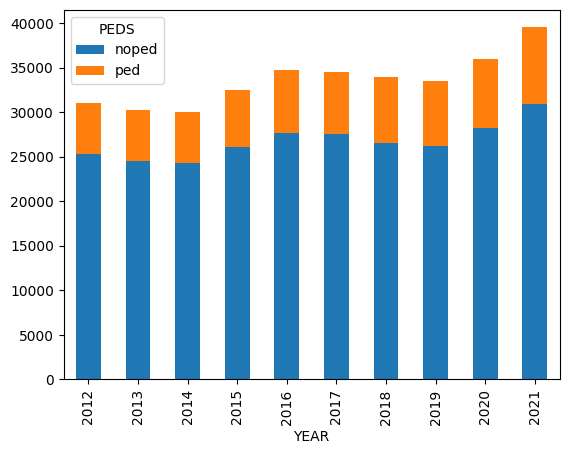
Create a stacked bar plot showing, for each year, the number of total accidents and (in a smaller bar, inside of the total one) accidents involving pedestrians.

If we have a series, a bar plot will show the index along the x axis, and the corresponding values in the heights of the bars.

If we have a data frame with two columns, then we’ll again see the index along the x axis. Each index will have two bars, one for each column.

If the two values can add up to a particular total, then instead of having them side by side, it might make sense to “stack” them. For this exercise, our goal is to create a data frame in which the years are the index, and we have two columns: One counting accidents without pedestrians, and another counting accidents with pedestrians.

We can use some similar techniques to what we did earlier, starting by with a “groupby” across years for the “PEDS” column, then running value_counts without normalize, giving us the raw number, and then unstack, which turns the number of injuries into columns:

(
    accident_df
    .groupby('YEAR')['PEDS']
    .value_counts()
    .unstack()
)

We get the following result:

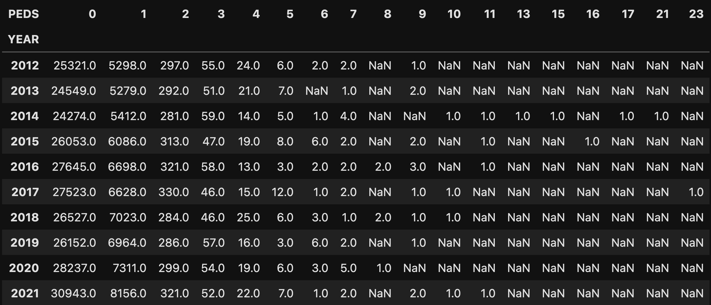
I now want to have a new column, “ped”, which totals all of the pedestrian-related accidents. I’ll do that by using “assign” along with lambda. The lambda will:

• remove the 0 column
• sum the remaining columns
• assign that sum to “ped”

Because all of this happens in the assign, it doesn’t affect the data frame permanently:

(
    accident_df
    .groupby('YEAR')['PEDS']
    .value_counts()
    .unstack()
    .assign(ped=lambda df_: df_.drop(0, axis='columns').sum(axis='columns'))
)

I then rename the 0 column to “noped”, and select just “noped” and “ped”. Then, finally, I call “plot.bar”, adding stacked=True so that it adds the bars together:

(
    accident_df
    .groupby('YEAR')['PEDS']
    .value_counts()
    .unstack()
    .assign(ped=lambda df_: df_.drop(0, axis='columns').sum(axis='columns'))
    .rename(columns={0:'noped'})
    [['noped', 'ped']]
    .plot.bar(stacked=True)
)

The result:

And that’s it for this week!

Here’s the Jupyter notebook that I used: https://drive.google.com/file/d/16JPRjn9enjDbseBRv4EkvWOHtK9HIxY4/view?usp=sharing

Questions, comments, or thoughts? Share them here!

I’ll be back on Wednesday with more puzzles about Python and Pandas based on current events.

Reuven