


This week, we’re looking at population data from the United Nations, in the wake of the declaration that India is the world’s most populous country, pushing China into second place. We’ll look at the most populous countries — both how they look now and how they’ll look in another decade — and will also examine fa
The population information and projections are all in a CSV file you can download from:
https://population.un.org/wpp/Download/Files/1_Indicators%20(Standard)/CSV_FILES/WPP2022_Demographic_Indicators_Medium.zipThis data set describes locations using ISO 3166 (https://en.wikipedia.org/wiki/ISO_3166-1), a standard for countries and regions. You can get those ISO codes on GitHub at
https://github.com/lukes/ISO-3166-Countries-with-Regional-CodesOr if you prefer to get the raw CSV data, you can get it from here:
https://raw.githubusercontent.com/lukes/ISO-3166-Countries-with-Regional-Codes/master/all/all.csvWith the data in hand, let’s move onto the analysis!
Retrieve the UN population data and projections, and put it into a data frame.
First and foremost, we need to load up Pandas:
import pandas as pd
from pandas import Series, DataFrame
%matplotlib inline
I first load Pandas up with the “pd” alias. And I load Series and DataFrame, because … well, because I always do, as a convenience. And because I’m working in Jupyter, and just in case Jupyter happens to not be configured to automatically show plots, I then use the magic command “%matplotlib inline” to show all plots inside of my Jupyter notebook.
With that, I start to load the data. One way to load it is to download the zipfile from the UN site, unzip it on my computer, and then to load it into a data frame with “read_csv”. But as you might know, read_csv can take a URL as an argument, meaning that instead of downloading the file first, I can just download it in real time. (This is less useful when the file is very large, of course.)
But wait: The URL that we’re downloading things from isn’t just a CSV file. It’s a zipped CSV file. And yet, it turns out that Pandas is just fine at downloading, unzipping, and then importing a zipped CSV file. It sees the “zip” suffix and does everything else automatically. I can thus say:
population_url = 'https://population.un.org/wpp/Download/Files/1_Indicators%20(Standard)/CSV_FILES/WPP2022_Demographic_Indicators_Medium.zip'

population_df = pd.read_csv(population_url, low_memory=False)
Notice that I passed the keyword argument “low_memory=False”. That’s because the data is large enough that Pandas is going to read it into memory in chunks. We don’t have to know or care about such chunking, except for the fact that Pandas also has to guess what dtypes we want for each of our columns. And guessing the dtype for each column is harder when you’re loading it in chunks.
One solution is to specify low_memory=False, which basically tells Pandas that it should feel free to read the whole file into memory at once. In that way, it can make an intelligent guess regarding how to classify the column, and assign it a dtype.
The other solution would be to specify a dtype for each column, passing a dictionary value to read_csv’s “dtype” keyword argument. That can certainly speed things up and lead to less ambiguity, but the first time I load a file into a data frame, I’m not prepared for such things.
Create a line plot showing the total world population (where "LocTypeName" is "World") across all years, including future projections. The x axis should be years, and the y axis should be population.
This sounds like a simple request, but it’s actually kind of complex!
First, we need to get the total world population from our data frame. It turns out that the data frame contains all sorts of population data mixed together — the whole world, individual countries, and regions are on different rows. And the population (data or projection) for each year is on a separate row, too.
We thus need to start by retrieving only those rows for which “LocTypeName” is set to “World”:
population_df.loc[population_df['LocTypeName'] == 'World']This is nice, but not quite enough to create our plot. The line plot we want has the years on the x axis, which means setting the years (the “Time” column) as the index to the data frame. And the data we want is the “TPopulation1July” column, the latest value that we can get for each year. (Population information is gathered or estimated twice each year, on January 1st and July 1st.)
I can thus take the above query, and use the two-argument version of .loc, meaning a row selector (just those rows for which LocTypeName is “World”) and a column selector (just the two columns Time and TPopulation1July:
population_df.loc[population_df['LocTypeName'] == 'World', ['Time','TPopulation1July']]Now that we’ve pared our data frame down to the rows and columns we need, we can take the “Time” column and turn it into the index:
population_df.loc[population_df['LocTypeName'] == 'World', ['Time','TPopulation1July']].set_index('Time')With that in place, we can finally create our plot:
population_df.loc[population_df['LocTypeName'] == 'World', ['Time','TPopulation1July']].set_index('Time').plot.line()This is what I get:
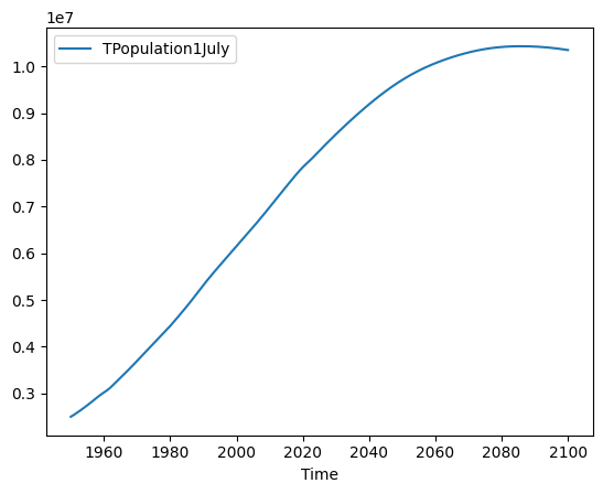
We can thus see that the world population is projected to continue growing for the next 50 years or so. But by the year 2100, growth will slow down, and maybe we’ll even start to see a decline in population. I’ve put it on my calendar for January 2100, to examine the data for Bamboo Weekly.
Retrieve the ISO location data, and put it into a separate data frame.
We’ve shown that we can work with the population data, which is fine. But if we want to start to work with countries and regions, we’ll need to load the country-name data, which is stored separately.
Why keep them separate? It’s part of an approach called “normalization,” common in the world of relational databases, in which we try to have each piece of data stored a single time. It’s the data version of the DRY (“don’t repeat yourself”) rule, allowing us to reference and update the data in a single place, rather than chase after it and in multiple places.
I decided to load this CSV data directly from a URL, as I did for the population data. I wasn’t sure if I really needed to say low_memory=False, but I set it anyway, just in case:
location_url = 'https://raw.githubusercontent.com/lukes/ISO-3166-Countries-with-Regional-Codes/master/all/all.csv'
location_df = pd.read_csv(location_url, low_memory=False)
Join the two data frames, so that we have access to both country names and projections in the same data frame.
I now have two data frames. The locations data frame contains all of the country names, as well as other info about each location (although we’ll basically ignore those). And the population data frame contains information about population, but doesn’t name any of the countries or regions.
We can combine them into a single data frame using a “join,” a common database operation that has been replicated in Pandas. This basically means telling Pandas that every row in location_df should be matched with a row from population_df, giving us a new data frame in which each row contains all of the columns from both data frames. (Yes, that’s a lot of columns!)
I didn’t say anything about what we should do if one of the rows doesn’t find any matches. That’s a whole other issue that we’ll deal with in another issue of Bamboo Weekly. For now, we can be confident that every location has population information, and that every row with population information matches a location.
The crucial question when joining two data frames together is: How do we know that two rows should be joined? We don’t want to do it via the indexes; it’s far from obvious (or true) that index 0 in location_df should be connected to index 0 population_df. And what if they aren’t the same size?
The solution is to find a column on in location_df that matches values in population_df. We can say that when there is a match, we can join the two rows together. We can do this in Pandas with the “merge” method. Whereas the better-known “join” method compares the indexes on the two data frames, merge lets us specify which column should be used on the left, and which should be used on the right.
In this case, the “country-code” column in location_df should be matched with the “LocID’ column in population_df. I thus run:
df = location_df.merge(population_df, left_on='country-code', right_on='LocID')The result is a new data frame, which we assign to “df”. Note that column names must always be unique in a data frame, so we’ll get an error if any names on the left and right data frames repeat. (In such cases, we have to tell Pandas what suffix we want to add to one or both data frames’ column names to avoid clashes.)
We now have a data frame with all of the information, including both population and country names. Just as the data was previously said to be normalized, we can say that the data is now denormalized, located in multiple places. That’s less efficient for storage and a bit harder for us to maintain, but it’s far easier to work with.
In 2023, what are the names and populations (as of July 1st) of the 10 most populous countries?
Once again, let’s break down how we’re going to find this information:
First, we need to find rows from 2023 (the current year).
Then we need to get just two columns, “name” (for the country name, originally from location_df) and “TPopulation1July” (for the current population, originally from population_df).
That’ll give us a new data frame back, with all countries and their current populations.
Then we can sort those rows by the population. Since the sorting will be from smallest to greatest population, we can grab the final 10 rows.
Let’s now walk through that process:
First, we’ll find rows from the 2023. Once again, we can use “.loc” to do that:
df.loc[df['Time'] == 2023]But since we only need two columns, we can use the two-argument version of “.loc”, passing a list of two columns we’re interested in:
df.loc[df['Time'] == 2023, ['name','TPopulation1July']]This returns a smaller data frame, one in which we have each country’s name and population in 2023. How can we find the most populous countries? We can sort the data frame by the “TPopulation1July” column.
But before we do that, let’s set the index to use the “name” column. That way, when we sort the values, the data frame’s index will be the country names, giving us a lot of flexibility:
df.loc[df['Time'] == 2023, ['name','TPopulation1July']].set_index('name').sort_values('TPopulation1July')The result is a one-column data frame in which the rows are sorted by TPopulation1July, from lowest to highest. I can grab the final 10 rows with the “tail(10)” method call. The end result is:
df.loc[df['Time'] == 2023, ['name','TPopulation1July']].set_index('name').sort_values('TPopulation1July').tail(10)And the 10 most populous countries? This is what I get:
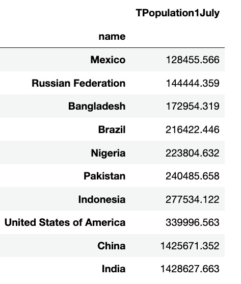
Sure enough, India has the biggest population, followed by China, the US, Indonesia, Pakistan, Nigeria, and Brazil. Finally, we see Bangladesh, Russia, and Mexico.
Note that the numbers here, like all of the population numbers in this data set, are in thousands. So when they say that there are 1,428,627.663 people in India, they really mean that there are 1,428,627,663 people there. And yes, this sounds extremely precise, but these are obviously estimates.
That’s why, when the news was announced about India’s population surpassing China’s, it was couched in estimates and predictions. It’s not like a big international counter rolled over, automatically detecting the point at which India became larger.
How much population are each of these countries expected to gain or lose in the coming 10 years (i.e., by 2023)?
Now that we know which are the 10 largest countries, we want to do some projections on them for the coming decade. How can we go about doing that?
For starters, we’ll need to grab rows for two different years, 2022 and 2023. We’ll only need three columns — “Time” (with the year), “name” (with the country name), and “TPopulation1July” (with the population). We can create that, once again, with “.loc” and using row and column selectors.
But wait — instead of using “==” to look for the years, I prefer to use “isin”, a great little method that lets us look for a value in a list of other values.
My total query, returning a smaller data frame, is thus:
df.loc[df['Time'].isin([2023, 2033]), ['Time', 'name','TPopulation1July']]It’s great that we got this data. But how can we turn it into a useful format for us to understand and compare populations?
My suggestion: A pivot table!
Pivot tables allows us to take row-by-row data and turn into two-dimensional data. It requires that we have two categorical columns and one numeric column. Here’s how I think about it:
- Distinct values of the “name” column, containing country names, will be our index, labeling the rows.
- Distinct values of the “Time” column, containing years, will be our index, labeling the columns.
- The values (“TPopulation1July”) will then be at the intersections of the columns and rows.
Here’s how we can do it:
df.loc[
    df['Time'].isin([2023, 2033]),
    ['Time', 'name','TPopulation1July']].pivot_table(index='name', columns='Time', values='TPopulation1July')
The result is great:
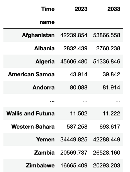
However, I’m only interested in the 10 most populous countries in 2023. I thus sort the results by the “2023” column, and take the 10 final values:
df.loc[df['Time'].isin([2023, 2033]), ['Time', 'name','TPopulation1July']].pivot_table(index='name', columns='Time', values='TPopulation1July').sort_values(2023).tail(10)This gives me the same values as before, plus a second column for 2033:
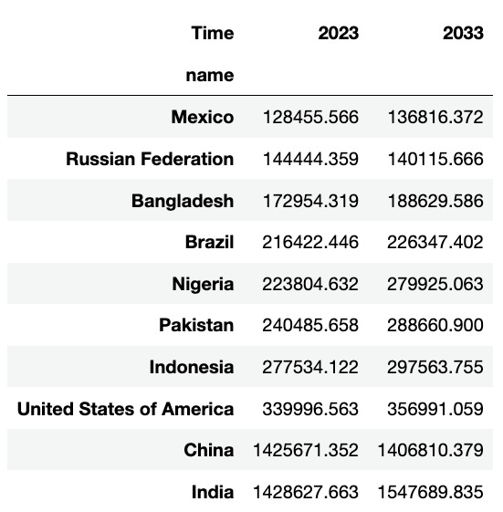
At this point, I want to know the difference between 2033 and 2033. Normally, I would use the “diff” method, but that works on rows. And I’m interested in comparing the columns.
Aha! It turns out that diff, like many methods in Pandas, takes an optional “axis” argument, allowing us to indicate in which direction the action should take place. We can specify “axis='columns'”, and it’ll do what we want.
Here’s the code I used:
df.loc[df['Time'].isin([2023, 2033]), ['Time', 'name','TPopulation1July']].pivot_table(index='name', columns='Time', values='TPopulation1July').sort_values(2023).tail(10).diff(axis='columns')And here’s the output:
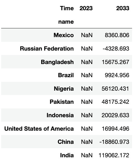
Notice that the 2023 column contains NaN values. When you run “diff”, the first column (or row, more usually) is always NaN, because it’s the baseline upon which all of these values run. The 2033 column is a bit more interesting, as we can see, so let’s grab just that:
df.loc[df['Time'].isin([2023, 2033]), ['Time', 'name','TPopulation1July']].pivot_table(index='name', columns='Time', values='TPopulation1July').sort_values(2023).tail(10).diff(axis='columns')[2033]The final output consists of these countries, and how much population they’ll gain or lose in another 10 years. The only two large countries that appear to be headed for a big decline in population are Russia and China.
For each of these countries, what are the migration rate and crude birth rate?
Why do countries gain or lose population? I’m not an expert, but I’m pretty sure that the two major factors are migration (in and out) and birth rates. (I’m guessing that health care and mortality rates also play a role!) The UN measures a variety of different birth rates, so we’re going to use their “crude” birth rate measure, just indicating how fast the population is growing via births.
I asked that for each of the largest countries, we look at their birth rates (“CBR”) and migration rates (“CNMR”) in 2023 and 2033. That will give us a sense of what’s happening in each of them.
Once again, I decided that it would be best to do a pivot table. Similar to before, I grabbed the rows from 2023 and 2033, and five columns: Time, name, TPopulation1July, CBR, and CNMR:
df.loc[df['Time'].isin([2023, 2033]), ['Time', 'name','TPopulation1July', 'CBR', 'CNMR']]But what sort of pivot table do I want to create? After all, I have too many values here to create a pivot table, no?
No, not if we use a multi-index! We can say that we’re interested in three different values for each row-column intersection:
df.loc[df['Time'].isin([2023, 2033]), ['Time', 'name','TPopulation1July', 'CBR', 'CNMR']].pivot_table(index='name', columns='Time', values=['TPopulation1July', 'CBR', 'CNMR'])The result looks like this:
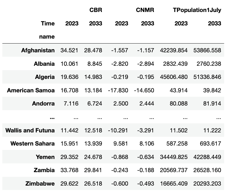
Now we just need to sort by the 2023 population and take the 10 largest countries. But… how do we sort by that column? How do we even reach that column, when it’s in a multi-index?
The answer: A tuple. If we pass a tuple to “sort_values”, Pandas is smart enough to see the first element as the first layer of the multi-index, and the second element as the second layer:
df.loc[df['Time'].isin([2023, 2033]),
    ['Time', 'name','TPopulation1July', 'CBR', 'CNMR']
   ].pivot_table(index='name',
                 columns='Time',
                 values=['TPopulation1July', 'CBR', 'CNMR']
  ).sort_values(('TPopulation1July', 2023)).tail(10)
Wow! That gives us exactly what we want:
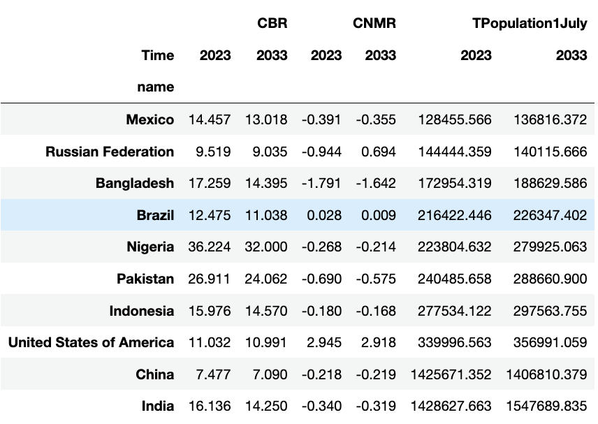
We can see that India and Indonesia have very high birth rates, but negative migration rates, and that both will remain that way in another 10 years. By contrast, China and Russia have low birth rates and negative migration. The US, meanwhile, has positive migration and decent (if not super high) birth rates.
Indeed, the only countries that seem to have positive migration in this entire chart are Brazil and the US.
Finally, what 10 countries have the highest birth rates in 2023? What 10 countries have the lowest birth rates?
I thought that it might be interesting to see which countries have the highest and lowest birth rates, given how important that is to a country’s growth.
What are the countries with the lowest birth rates, at least in 2023? I can calculate that with:
df.loc[df['Time'] == 2023, ['name', 'CBR']].set_index('name').sort_values('CBR').head(10)I grab the “Time” and “CBR” columns, limit Time to be the year 2023, set the country name to be the index, and sort values by CBR. The 10 smallest-growing countries are:
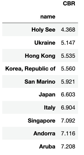
I mean, I guess it’s kind of obvious why the Vatican (“Holy See”) doesn’t have high birth rates, right? I had heard that there are very low birth rates in Korea, Japan, and Italy, but didn’t realize just how low they are.
What about on the high side? I can recreate my query, but substituting “tail(10)”:
df.loc[df['Time'] == 2023, ['name', 'CBR']].set_index('name').sort_values('CBR').tail(10)And the baby winners are:
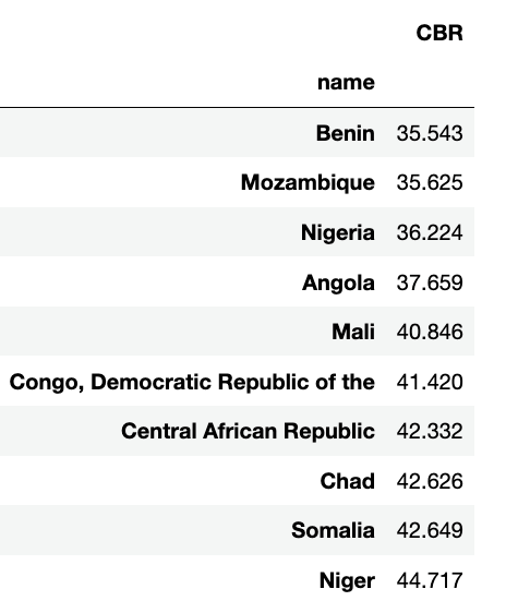
Wow, that’s a lot of births! I must admit that I’m so used to hearing that Israel has a high birth rate that I was half expecting it to be there. But no, we’re only at 19.047, a very far cry from these other countries — even if it’s far higher than many European countries.
I hope that this was interesting and fun! Please post any suggestions, corrections, and comments below.
Here’s my Jupyter notebook for the week: https://drive.google.com/file/d/1a-kS80lkfhi7M5zzJ9nah5EoVAplCvMt/view?usp=drive_link
I’ll be back next week, with another Pandas problem related to the news.
Reuven